Week 5: Static Clustering Pipeline

The Static Clustering Pipeline

Key Points Driving the Pipeline

Let us recall the key issues we want to address in our new pipeline, detailed in the last post:

• Pull out richer GDELT info
• Cluster on news-topic-related information (this is really the core of our hypothesis of prediction by GDELT).
• Represent non-orthogonal column relationships
• Manage high volumes of data: use strategies to increase parallelism and minimize the serial bottlenecks without sacrificing too much accuracy.

High-level structure

The data has several stages (numbers below are accurate to within the order of magnitude). Data is stored in a TSV ASCII format.

Preprocess refers to extracting and sanitizing relevant GDELT features.

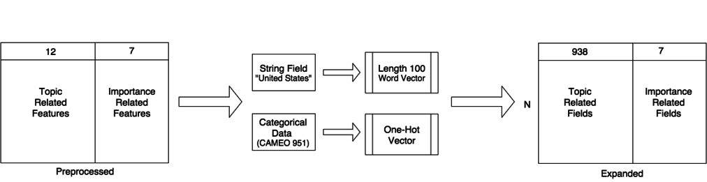
Expanding refers to transforming the preprocessed data into wide numerical feature vectors.

Clustering refers to classifying expanded data according to a \(K\)-means model. This model is computed beforehand from a static random sample of our data.

Conglomeration coalesces a day’s data, in a manner that will be described shortly.

We parallelized usually to the maximum possible on cycles.cs.princeton.edu: 48. Parallelizing along the following for-loops:

To learn the \(K\)-means, we first perform for each day:

1. Random sample each day with equal number of rows
2. Preprocess
3. Expand

Then for each \(K\), learn a mini-batch-based \(K\)-means on the concatenated output from (3), above.

For the actual regression, for each day, we:

1. Preprocess
2. Expand
3. Cluster and Conglomerate

Finally, for each set of GLM hyper paramters, we learn and validate on the concatenated output of (3) from above.

Preprocessing stage

Raw data: 58 columns, mixed types

Preprocessed data: 19 columns, numeric, categorical, or string (coming soon!). Categorical values are represented as integers in \([1, N]\), with 0 representing an empty cell. When expanded to the one-hot encoding, 0 doesn’t get its own value (it’d be wrong to learn off missing data - or is it?).

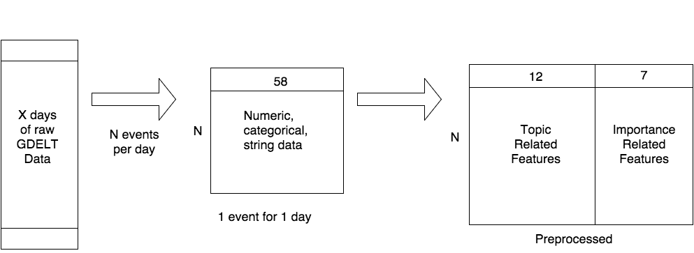
Expansion stage

Expanded data: 945 columns, all numeric.

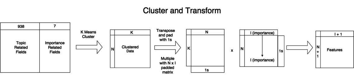
Cluster stage

Coalesced data: 1 row, \((K+1)(I+1)\) columns, where \(I\) is the number of “importance-related” columns (note minor typo in last stage below).

Label data: Time series of prices. We generate day-to-day diffs from this. It’s small enough to fit in memory and generate on the fly.

Importantly, we divide each day’s summary vector (the result of the matrix multiply and subsequent flatten) by the number of rows \(N\) for that day, so days aren’t skewed by event counts (consider the final constant column).

Generalized Linear Model

Currently a logistic classifier. Hyper parameters are regression (\(L_1,L_2\)), \(K\), and regularization coefficient.

Data Used

Clusters learned from random sample of 20130401-20150731, 150 lines per day. 200MB, 120K lines total. Each clustering model (for different \(K\)) takes between 1-50MB.

Raw data 20130401-20151021 (a few extra months to test on data that didn’t affect the random sample for clustering). 60GB total. Coalesced day-summaries (acutally used for regressions) take up 5-200MB, depending on \(K\).

Results

We tested our GLM predictions on silver (XAG) commodity pricing data.

Our date range of 20130401-20150731 containing 172 days was split into a training set containing 88 days, a validation set containing 30 days, and a test set containing 50 days.

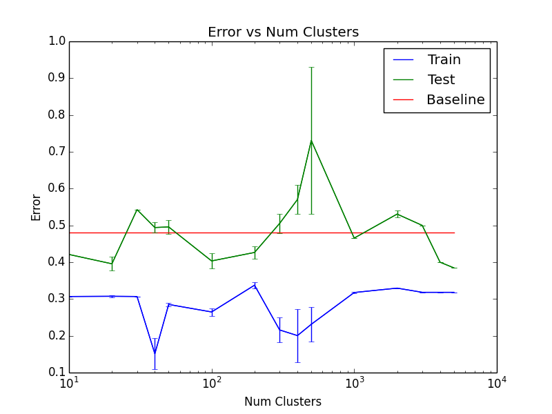
For baseline values, 58 of 80 train days had prices go down, as did 19 of 30 validation days and 26 of 50 test days. Thus the baseline error for predicting 0 on every day would have been \(24/50=0.48\).

We trained 54 logistic regression models, varying the number of clusters trained on, the inverse regularization strength \(c\), and the type of regularization (\(L1\) or \(L2\)).

\[K = \{10, 20, 30, 40, 50, 100, 200, 300, 400, 500, 1000, 2000, 3000, 4000, 5000\}\] \[c = \{0.01 - 0.1, 0.1 - 1, 1 - 10\}\]

We also tested precision, recall, and f1 scores for various prediction probability cutoffs between 0.1 and 0.9.

The model with the least error was trained on \(K=5000\), \(c=2\), and used \(L1\) regularization.

Training Accuracy: 0.682

Test Accuracy: 0.615

Precisions:

• 0.10: 0.85
• 0.25: 0.85
• 0.50: 0.70
• 0.75: 0.85
• 0.90: 0.85

Recalls:

• 0.10: 1.00
• 0.25: 1.00
• 0.50: 0.44
• 0.75: 0.00
• 0.90: 0.00

F1:

• 0.10: 0.82
• 0.25: 0.82
• 0.50: 0.50
• 0.75: 0.00
• 0.90: 0.00

Overall train and test errors as a function of \(K\) can be seen here. Models were retrained 20 times each.

NOTE FOR FULL DISCLOSURE: We computed the clusters on the a large part of dataset, but due to time constraints had to run initial predictions on the subset of the data that was clustered and coalesced, which did not at the time include the few most recent months reserved for testing. As a result, test data was used for computing K-means. We think this may inflate test accuracy slightly. However, the clusters were also computed from samples of days far in the future of the test data, so those likely had a cancelling adverse effect. In any case, these initial exploratory results are just hints at a possible signal.

Future Work

Multicomputer parallelism

The above pipeline, run on one machine with 48 CPUs, handled \(\frac{3}{4}\) of a year’s worth of data in 8 hours (as of the writing of this post, it’s still going).

As we change our feature extraction methods from the raw data (see below), iterative updates to the day-summaries need to be expedited.

First priority is to get the sampling and clustering pipelines (mainly the latter) running on a beowulf cluster, ionic.cs.princeton.edu, with about 500 accessible CPUs. This will get us down to about \(1\) hour per year of data - still not too great, we could go up to about 900, at one CPU per day.

Word2Vec

Word2Vec is an unsupervised learning algorithm that finds a mapping from words or phrases to \(\mathbb{R}^D\) for a set parameter \(D\). This is done by initializing randomly, and then updating tokens’ word vectors (words or phrases, as identified by a frequency-based bigram/trigram/quadgram model) with linear combinations of surrounding tokens’ current word vectors according to the corpus.

We initially tried Brown’s NLTK corpus with quadgrams. Unfortunately, common actor names, like ‘singapore’ or ‘protester’ were not present in the corpus.

After we expand the corpus to a larger (still static) one, we can utilize some of GDELT’s string column features by expanding them to \(\mathbb{R}^D\) in the expand phase.

An interesting alternative is to use a dynamic corpus, learning off of the GDELT news articles themselves (involves scraping the URLs).

Normalization and scale

Currently, the topic-columns are not scaled to their z-scores (the per-day parallelism would break down if we computed the data-set-wide \(\mu,\sigma\)). This negatively impacts clustering because high-magnitude columns dominate distance.

Possible solution: A preferable alternative is to rely on the manageable size of the random sample we learn the clusters from. Prior to fitting K-Means, we can compute \(\hat{\mu},\hat{\sigma}\) from the sample itself. Then we compute the z-scores for each column.

Question: do we need to be careful to use an unbiased estimator for \(\sigma\)? This isn’t a true random sample anyway, would the correction even make sense? The point is just to scale the values to reasonable ranges.

Periodicity features

Consider adding features like \(\sin \frac{d}{2\pi P}\) or \(d % P\) to capture periodicity.

Question: How to learn \(P\)? As a hyperparameter, or is there a more intelligent way.

More stuff

1. Smarter clustering: Don’t create a sparse binary matrix of clustered news, create a matrix of posteriors for a news-GMM.
2. Nonparametric clustering: Infinite GMM, HDP, SNΓP
3. Other classifiers: SVM
4. Linear regression on \(\frac{p_{t+1}-p_t}{p_t}\).
5. Try other commodities, try older data.

The most up-to-date TODO list is in the README in the repo.