Week 6: Trying out new approaches
SLURM Integration
Using ionic cluster with SLURM scheduling script, we can increase the number of processors for our day-summary pipeline. This took a lot of annoying sysadmin work (libc version was different between cluster computers), but in the end was very successful.
Note that below the Expansion stages include Preprocessing, see the previous post for details of what each stage does.
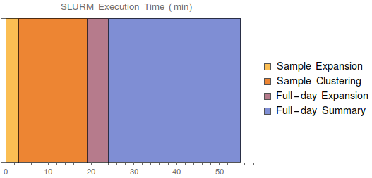
End to end runtime: 55 minutes! Much less than cycles-only, which was more than 1.5 days.
Still could take advantage of more parallelism, but the next steps up (Della/Hecate/Orbital/Tiger clusters) are generally hidden from undergrads. We’ll probably stick to ionic.
Future improvements
- Can parallelize sample expansion and learning with full-day expansion
- Make some easy optimizations to the Python code itself soe we can run more processes at the same time (bottlenecked by memory usage)
- Nicer error handling.
Changes to the Pipeline
Word2Vec representation of actor names
We trained a Word2Vec model with window size 5 on The Europarl parallel corpus, which is the extracted proceedings of the European Parliament 1994 to 2011. It contains 53.9M words in 2.2M sentences and covers topics such as politics, agriculture, economics, military and science. We used this W2V model to represent actor names as a real-valued vector in which PMI information is encoded.
Results of using word vectors for actor names
Entity recognition in excess of 90%, will try t o re-run with the added w2v models.
K-Means to Infinite GMM
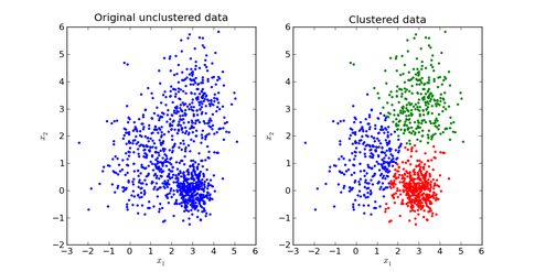
\(K\)-means defines hard clusters GMMs are appealing because GMMs will generalize clustering to use information about the covariance of the data
Still, with GMMs and \(K\)-Means clustering, we need to do a parameter search for the number of \(K\) clusters (or mixture components)
Don’t have any intuitive sense for how many news clusters there are Very hard to guess with 200k news events a day
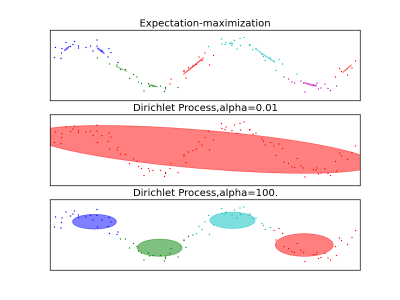
Use infinite GMM (DPGMM) Gaussian mixture model with Dirichlet process prior defined over mixture components Predicts number of clusters while performing model inference Number of clusters change to fit data Works well when clusters are approximately Gaussian and well-defined Not as good when distributions of clusters are skewed or tailed
Implementation uses \(\alpha\) parameter for cluster hyperparameter Set at 1 (Rasmussen uses 3.5) Has \(N\) to limit the maximum number of components \(N=5000\) since we want to approximate an infinite model
Time Series Analysis
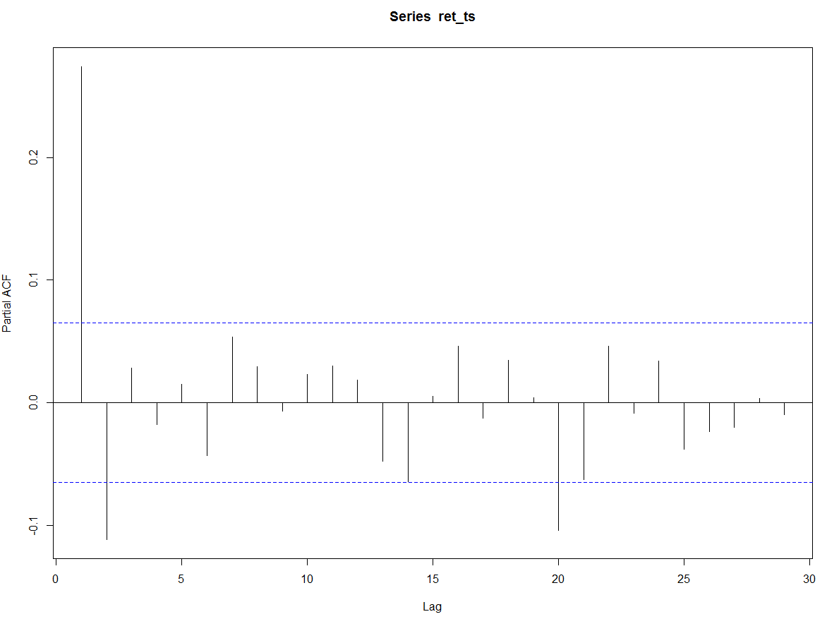
Exploration of the new time series: XAG = Silver Ounce Rates

We started by exploring the PACF graph to understand the autocorrelations between the lags and we found the following graph. This graph demonstrates that at any point in the time series, the value is correlated with the value at lags: 1, 20, 41, 49, 87, 100… We could also have seasonality given the range of the autocorrelated lags but none of the standard forecast() R libraries managed to confirm the seasonality of the time series (tbats(x) returned a NULL period).

Fitting with a fixed window + AIC/Likelihood/Significance measures:
Variable Selection:
The variables we would be considering in any kind of AutoRegressive model are mainly the lags and the exogenous regressors. For more advanced AutoRegressive models, we also have the parameters for drift, moving average, integration factor and seasonality period.
Picking Lags:
Giving the PACF, we have an idea of the lags we would be considering for modeling our time series. A classic approach would be to fit a linear model of the different lags as independent variables and identifying which lags lead to the lowest AIC. Additionally, the statistical significance of the specific lags can be a good indication. By selecting long lags with several of them set to zero (picking 1 and 20 but nothing in between), we’re using “subset ARIMA”. As a matter of fact, with more observations (the larger the window), the less dependent are the ensuing forecasts on the previous forecasts (in a recursive fashion) leading to more of a direct forecasting than direct forecasting. Several works have demonstrated thast the loss of efficiency due to using fewer observations generally does more harm than the potential bias improvements due to forecasting directly.
Selecting columns from the preprocessed news data:
We are proposing our own implementation of a bottom-up stepwise addition of vectors (separate regressors in this case) to the AR model (could be ARIMA). Accordingly, we would start by fitting the model including all the exogenous regressors and getting the corresponding t-statistics. We would then sort the regressors by the magnitude of the t-statistic (in absolute value: the greater the more statistically significant). Consequently, we fit the AR model including only the regressor with the highest t-statistic in absolute value. If it is significant, we conider it towards our final set of regressors, otherwise, discard it. We repeat the previous step by considering regressors in order and including them only if they are stil significant when inserted into the final set of regressors. This would also help avoiding potential multicolinearity problems. These problems could arise if two topics are complementary, for example.
AIC: 745
Multiple R-squared: 0.9835, Adjusted R-squared: 0.5266
F-statistic: 2.153 on 803 and 29 DF, p-value: 0.006709
Forecast Evaluation with a rolling origin/moving window:
[forecast calculations: h-step forecasts use the preceding 1:(h-1)-step forecasts for AR(1)]
Error Measure:
We’re currently using the Mean Absolute Error (MAE) to quantify the error rate of our predictions. However, as discussed earlier (and unfortunately still not implemented) we’re leaning towards adopting an measure similar to the Information Ratio in the future. Accordingly, our evaluation of the forecasting would be binary, at each day the forecasting is correct if the forecast is in the same direction as the actual value with respect to the moving average (or start of the window) and if the difference in magnitudes is greater than a certain threshold (determined by the volatility over a given number of recent days).
Trading Strategy:
Given that our main goal is not only to build a statistically robust model but to also be able to build a trading strategy out of it. For the testing, we’re considering using Quantopian for evaluating our trading algorithm.
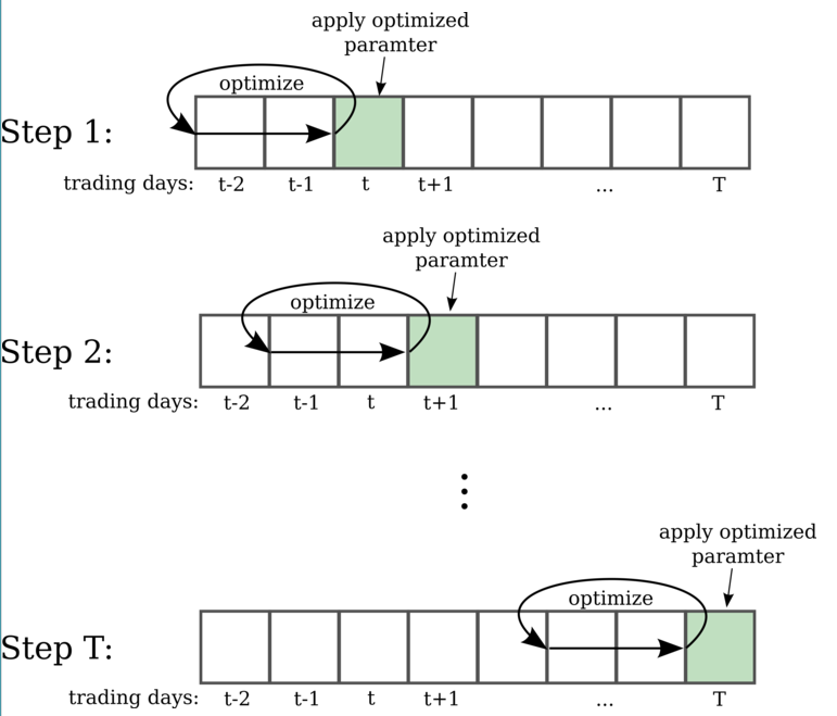
Rolling Origin/Walk forward optimization: Cross-Validation for Time Series:
Assume you need at least k observations to produce a reliable forecast(need last 5 lags for the AutoRegressive model, for example) The way it works is by setting an origin (k+i-1) based on which the forecast rolls foreward in time. At each i (from 1 to T-k), we use the observations at time 1->k+i-1 to estimate the forecasting model and compute the error on the forecast for time k+i: One-Step Forecast.
However, one-step might not be as relevant as multi-step (e.g. long-term trading strategies). In that case, rolling forecasting origin can be modified to allow multi-step errors to be calculated. In that case, if we were to compute h-step-ahead forecasts, our origin would be k+h+i-1. We would use the observations from 1 to k+i-1 in order to estimate the forecasting model and compute the h-step error on the forecast for time k+h+i-1. Depending on the AR model, the h-step-ahead could be fully dependent on the observations or be a recursive forecast.
This optimization method allows us to apply our trading strategy in real time as it continues to lear as new data becomes available. Additionally, it adapts to changes in the markets instead of being anchored to old time series data.
 Eventually, we will have to deal with evaluating K as a hyperparameter: how many days do we need to look back to for the training. As for h, it can be evaluated for any model based on the imminen increase of test error as h increases.
Logistic Regression and SVM
Previously, we used logistic regression to predict the price movements for silver. We ran our models on a training set containing 88 days, a validation set containing 30 days, and a test set containing 50 days.
The test accuracy as a function of \(K\) for the best parameters can be seen here:
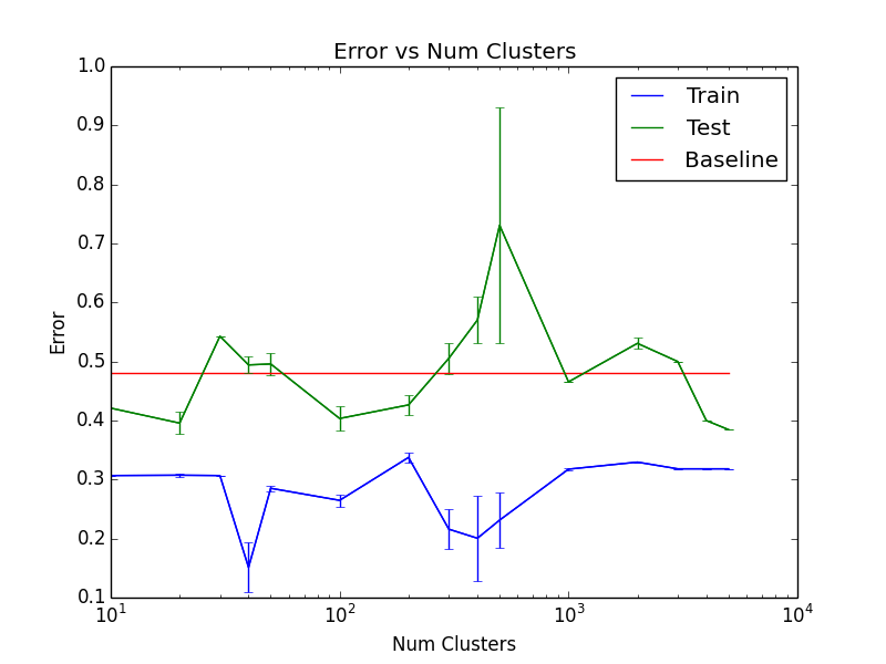
Since this is not very convincing that our model outperforms the benchmark, we expanded our date range to 20130401-20151001. There were 526 days for training, 207 days for validation and 152 days for testing. Out of the 152 days, the prices increased in 58 days (61.8% of the days were decreasing).
We performed logistic regression with L1 and L2 regularization with different regularization weights in [0.01, 1000].
We also reduced the number of dimensions with PCA and performed SVM with error penalties in [0.01, 1000] with different kernels on the data.
We pick the parameters that produce the highest accuracy on the validation set and calculate the accuracy on the test dataset. The best models from both logistic regression and SVM only produced the same accuracy as the bestline on the test set (guessing that every day goes down).