A Modeling Introduction to Deep Learning

In this post, I’d like to introduce you to some basic concepts of deep learning (DL) from a modeling perspective. I’ve tended to stay away from “intro” style blog posts because:

There are so, so many of them.
They’re hard to keep in focus.

That said, I was presenting on BERT for a discussion group at work. This was our first DL paper, so I needed to warm-start a technical audience with a no-frills intro to modeling with deep nets. So here we are, trying to focus what this post will be:

It will presume a technically sophisticated reader.
No machine learning (ML) background is assumed.
The main goal is to set the stage for future discussion about BERT.

Basically, this is me typing up those notes. Note the above leaves questions about optimization and generalization squarely out of scope.

The Parametric Model

Deep learning is a tool for the generic task of parametric modeling. Parametric modeling (PM) is a term I am generously applying from statistical estimation theory that encapsulates a broad variety of ML buzzwords, including supervised, unsupervised, reinforcement, and transfer learning.

In the most general sense, a parametric model \(M\) accepts some vector of parameters \(\theta\) and describes some structure in a random process. Goodness, what does that mean?

Structure in a random process is everything that differentiates it from noise. But what’s “noise”?
When we fix the model \(M\), we’re basically saying there’s only some classes of structure we’re going to represent, and everything else is what we consider noise.
The goal is to pick a “good” model and find parameters for it.

A Simple Example

For instance, let’s take a simple random process, iid draws from the normal distribution \(z\sim \mathcal{D}= N(\mu, \sigma^2)\) with an unknown mean \(\mu\) and variance \(\sigma^2\). We’re going to try capture the richest possible structure over \(z\), its actual distribution. One model might be the unit normal, \(M(\theta)=N(\theta, 1)\). Then our setup, and potential sources of error, look like this:

sources of error

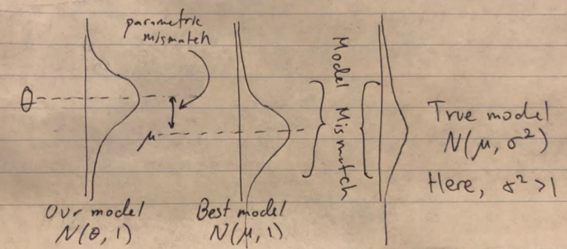
What I call parametric and model mismatch are also known as estimation and approximation error (Bottou and Bousquet 2007).

Here, we have one the most straightforward instances of PM, parameter estimation (we’re trying to estimate \(\mu\)).

Revisiting our definitions

What constitutes a “good” model? Above, we probably want to call models with \(\theta\) near \(\mu\) good ones. But in other cases, it’s not so obvious what makes a good model.

One of the challenges in modeling in general is articulating what we want. This is done through a loss function \(\ell\), where want models with small losses. In other words, we’d like to find a model \(M\) and related parameters \(\theta\) where \[ \E_{z\sim \mathcal{D}}\ha{\ell(z, M(\theta))} \] is as small as possible (here, for our iid process). Note that in some cases, this doesn’t have to be the same as the loss function used for optimization for finding \(\theta\), but that’s another discussion (there are several reasons to do so).

Another Example

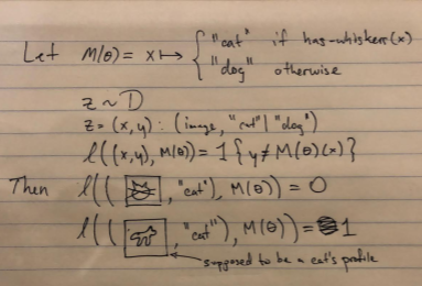
Now let’s jump into another modeling task, supervised learning. Here:

Our iid random process \(\mathcal{D}\) will be generating pairs \(\pa{\text{some image}, \text{“cat” or “dog”}}\).
The structure we want to capture is that all images of dogs happen to be paired with the label \(\text{“dog”}\) and analogously so for cats.
We’ll gloss over what our model is for now.

A loss that captures what we want for our desired structure would be the zero-one loss, which is \(1\) when we’re wrong, \(0\) when we’re right. Let’s fix some model and parameters, which takes an image and labels it as a cat or dog (so \(M(\theta)\) is a function itself) as follows, and then let’s see how it does on our loss function.

sources of error

OK, so why Deep Learning?

This post was intentionally structured in a way that takes the attention away from DL. DL is a means to achieve the above PM goals–it’s a means to an end and being able to reason about higher-level modeling concerns is crucial to understanding the tool.

So, DL is an approach to building models \(M\) and it studies how to find good parameters \(\theta\) for those models.

Deep Learning Models

A DL model is anything that vaguely resembles the following model. Namely, it has many parameterized functions composed together to create a function.

A function is usually good enough to capture most structure that we’re interested in random processes, given sufficiently sophisticated inputs and outputs. The inputs and outputs to this function can be (not exhaustive):

fixed-width multidimensional arrays (casually known as tensors, sort of)
embeddings (numerical translations) of categories (like all the words in the English dictionary)
variable width tensors

The parameters this function takes (which differ from its inputs and effect what the function looks like) are fixed width tensors. I haven’t seen variable-width parameters in DL models, except as some Bayesian interpretations (Hinton 1993).

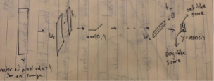
The Multi-Layer Perceptron

Our prototypical example of a neural network is the Multi-Layer Perceptron, or MLP, which takes a numerical vector input to a numerical vector output. For a parameter vector \(\theta=\mat{\theta_1& \theta_2&\cdots&\theta_L}\), which contains parameters for our \(L\) layers, an MLP looks like: \[ M(\theta)= x\mapsto f_{\theta_L}^{(L)}\circ f_{\theta_{L-1}}^{(L-1)}\circ\cdots\circ f_{\theta_1}^{(1)}(x)\,, \] and we define each layer as \[ f_{\theta_i}=\max(0, W_ix+b_i)\,. \] The parameters \(W_i, b_i\) are set by the contents of \(\theta_i\).

This is the functional form of linear transforms followed by nonlinearities. It describes what’s going on in this image:

sources of error

Why DL?

While it might be believable that functions in general make for great models that could capture structure in a lot of phenomena, why have these particular parameterizations of functions taken off recently?

This is basically the only part of this post that has to do with DL, and most of it’s out of scope.

In my opinion, it boils down to three things.

Deep learning is simultaneously:

Flexible in terms of how many functions it can represent for a fixed parameter size.
Lets us find so-called low-loss estimates of \(\theta\) fairly quickly.
Has working regularization strategies.

Flexibility

The MLP format above might seem strange, but this linearity-followed-by-non-linearity happens to be particularly expressive, in terms of the number of different functions we can represent with a small set of parameters.

The fact that a sufficiently wide neural network can well-approximate smooth functions is well known (Universal Approximation Theorem), but what’s of particular interest is how linear increases in depth to a network exponentially increase its expressiveness (Montúfar, et al 2014).

expressiveness

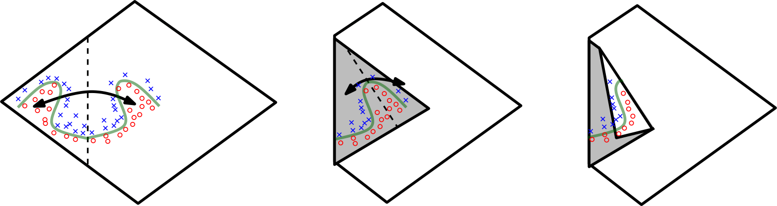
An image from the cited work above demonstrates how composition with non-linearities increases expressiveness. Here, with an absolute value nonlinearity, we can reflect the input space on itself through composition. This means we double the number of linear regions in our neural net by adding a layer.

Efficiency

One of the papers that kicked off the DL craze was Alexnet (Krizhevsky 2012), and the reasons for its existence was that we could efficiently compute the value of a neural network \(M(\theta)\) on a particular image \(x\) using specialized hardware.

Not only does the simple composition of simple functions enable fast forward computation of the model value \(M(\theta)(x)\), but because the operations can be expressed as a directed acyclic graph of almost differentiable functions, one can quickly compute reverse automatic derivatives \(\partial_\theta M(\theta)(x)\) in just about the same amount of time.

This is a very happy coincidence. We can compute the functional value of a neural net and its derivative in time linear in the parameter size, and we have a lot of parameters. Here, efficiency matters a lot for the inner loop of the optimization (which uses derivatives with SGD) to find “good” parameters \(\theta\). This efficiency, in turn, enabled a lot of successful research.

Generalization

Finally, neural networks generalize well. This means that given a training set of examples, they are somehow able to have low loss on unseen examples coming from the same random process, just by training on a (possibly altered, or regularized) loss from given examples.

This is particularly counterintuitive for nets due to their expressivity, which is typically at odds with generalization with traditional ML analyses.

have been proposed, but none of them are completely satisfying yet.