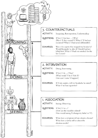
If you read Judea Pearl’s The Book of Why, it makes it seem like exercising observational statistics makes you an ignoramus. Look at the stupid robot:

Pearl and Jonas Peters (in Elements of Causal Inference) both make a strong distinction, it seems at the physical level, between causal and statistical learning. Correlation is not causation, as it goes.

From a deeply (Berkeley-like) skeptical lens, where all that we can be sure of is what we observe, it seems that we nonetheless can recover nice properties of causal modeling even as associative machines through something we can call the Epistemic Backstep.

This is of less of a declaration of me knowing better, and more of an attempt at trying to put into words a different take I had as I was reading the aforementioned works.

Our Shining Example

Intuitively, the difference between cause and effect seems to be a fundamental property of nature. Let \(B\) be barometric pressure and \(G\) be a pressure gauge’s reading. We can build a structural causal model (SCM), which is some equations which are tied to the edges and vertices of a directed acyclic graph (DAG): \[ B\rightarrow G \] where \(B\) is the cause and \(G\) is the effect. It’s clear to us that the former is a cause because of what interventions do.

If we intervene on \(B\), say, by increasing our elevation, then the gauge starts reading a lower number. There’s clearly a functional dependence there (or a statistical one, say, in the presence of measurement noise).

If we intervene on \(G\), by breaking the glass and turning the measurement needle, our eardrums don’t pop no matter how low we turn the needle.

We point at this asymmetry and say, this is causality in the real world.

The Epistemic Backstep

But now I ask us to take a step back. Why does this example even make sense to us, evoking vivid imagery about how ridiculous a ruptured eardrum would be due to manually changing a barometer’s needle?

Well, it turns out that we have, through media or real-life experiences, learned about and observed barometers. In science class, we may have read about or seen or heard how they turn as pressure changes.

We may never have broken a barometer and changed its needle position, but we’ve certainly seen enough glass being broken in the past and needles moving that we can put two and two together and imagine what that would look like. In those situations, the thing that the needle measures rarely changes.

Stepping back a bit, it turns out that we actually have a lot of observations of some kind of environmental characteristic \(C\) (which might be temperature or pressure), its corresponding entailment \(E\) (a thermometer or barometer reading), and a possible interaction with the measurement took place, \(I\), where here this represents an indicator for “did we increase the reading of our measurement manually.”

So, we actually have a lot of observational evidence of the more generalized system \((C, E, I)\).

1. We’ve seen how barometers read high numbers \(E=1\) at high pressure \(C=1\) by being at low altitude and observing a functioning barometer. We did not mess with the barometer. \((C, E, I)=(1, 1, 0)\).
2. We’ve seen how barometers behave at high altitude \((0, 0, 0)\).
3. We’ve seen how ovens increase the temperature in the attached thermometer \((1, 1, 0)\).
4. How we don’t have a fever if our mom measures our temperature and we’re healthy \((0, 0, 0)\).
5. After we do jumping jacks to raise our temperature, to get out of school, we see that it works \((0, 1, 1)\).

Given a bunch of situations like this, and taking some liberty in our ability to generalize here, it’s totally reasonable we can come up with a rule \(E=\max(C, I)\) and given observational data alone. We might go even further, and model a joint probability on \((C, E, I)\) where the conditional probability distribution of \(C\) given \(E=1,I=1\) ends up just being the marginal probability of \(C\): \[ p(C) = p(C|E=1,I=1)\,, \] as opposed to what happens for \(E\) \[ \forall i\,,\,\,\,p(E|C=1, I = i) = 1_{E=1}\,. \] These observations make for natural matches for causal inference, from which we can infer that there won’t be much effect on pressure by changing the barometer, but we could have known this (at least in theory) just by building up an associative model for what happens when you manually override what the measurement tool says.

By considering the associative model over a wider universe, a universe that includes the interventions themselves as observed variables, and having a strong ability to generalize between related interventions and settings, we can view our causal inference as solely an associative one.

In Short

The epistemic backstep proceeds by adding a new variable, \(F\), for “did you fuck with the system you’re modeling,” capturing all the essential ways in which you can fuck with it, and in this manner we can seemingly reduce causal questions to those that in theory an associative machine could answer.

Maybe this is a cheap move, just moving intervention into the arena of observations. I still think it’s a fairly powerful reduction: we can tell things about gauges and barometers having never experimented with them before, as long as we can solve the transfer learning problem between those and settings where we have messed with measuring natural phenomena, maybe thinking back to weight scales in a farmer’s market or trying to get out of school by raising our temperature.

So, we can view randomized controlled trials in this context not as different experimental settings, but rather a way to collect data in a region of the \((C, E, I)\) space that might be sparsely populated otherwise (so we’d have a tough time fitting the data there).

It’s important to note that it doesn’t matter that it’s more convenient for us to model causal inference with DAGs.

• You may say something like “well, how did you know that jumping jacks would help raise your temperature?”
• This suggests that humans do really think causally.
• However, the above is a psychological claim about humans, rather than a metaphysical claim about causality.
• For all we know, an associative machine may have an exploration policy where, on some days, it sets \(I=1\) just to see what can happen. After gathering some data, it builds something equivalent to a causal model, but without ever explicitly constructing any DAGs.

Full Circle

For what it’s worth, maybe the best way to model our new joint density \((C, E, I)\) is by first identifying the causal DAG structure, constructing a full SCM by fitting conditional functions, and then using that SCM for our predictions.

But that seems presumptuous. Surely, viewing this as a more abstract statistical learning problem, there might be more generic ways of finding representations that help us efficiently learn the “full joint” which includes interventions.

Another interesting point is asking questions about counterfactuals. Personally, I don’t find counterfactuals that useful (unless blame is an end in itself), but that’s a discussion for another time. I didn’t want to muddy the waters above, but there’s an example of an associative counterfactual analysis below with the epistemic backstep.

Note that the transfer notions introduced here aren’t related to the Tian and Pearl transportability between different environments, where the nodes of your SCM stay the same (see here for further developments). What I’m talking about is definitely more of a transfer learning problem, where you’re trying to perform a natural matching based on your past experiences, and it’s learning this matching function that’s interesting to study.

So in sum we have an interesting take on Regularity Theory, which doesn’t have the usual drawbacks. Maybe all of this is a grand exercise in identifying a motivation for Robins’ G-estimation. In any case it was fun to think about so here we are.

Another worked example

Let’s first look at Pearl’s firing squad.

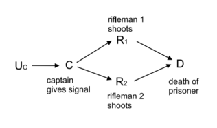
Say the captain gave the order to fire, both \(R_1,R_2\) did so, and the prisoner died. Now, what would have happened had \(R_1\) not fired?

Pearl says the association machine breaks down here, it’s a contradiction, since the rifleman always fires when the captain gives the order to. So why aren’t we confused when we think about it?

Step back: consider a universe where riflemen can refuse to follow orders. The first rifleman is now wont to be mutinous \(M\) (add an arrow \(M\rightarrow R_1\)).

In situations, where the first rifleman is mutinous, but the second isn’t, it’s pretty clear what’ll happen. The second rifleman still fires, and the prisoner is still shot dead.

To me, it’s only because I’ve seen a lot of movies, read books, heard poems where there’s a duty to disobey that I could reason through this. If all of my experience up to this point has confirmed that riflemen always fire when their commanding officer tells them to, I would’ve been as confused as our associative machine at the counterfactual question.

To close up, we have one big happy joint model \[ p(C, M, R_1, R_2, D)\,, \] now so to ask the counterfactual is just to ask what the value of \[ p(D=1|C=1, M=1, R_1=0, R_2=1) \] is, which is something we can answer given our wider set of observations and the ability to generalize.