Multiplicative weights is a simple, randomized algorithm for picking an option among \(n\) choices against an adversarial environment.
The algorithm has widespread applications, but its analysis frequently introduces a learning rate parameter, \(\epsilon\), which we’ll be trying to get rid of.
In this first post, we introduce multiplicative weights and make some practical observations. We follow Arora’s survey for the most part.
Problem Setting
We play \(T\) rounds. On the \(t\)-th round, the player is to make a (possibly randomized) choice \(I_t\in[n]\), and then observes the losses for all of the choices, the vector \(M_{\cdot, j_t}\), corresponding to the \(j_t\)-th column of a matrix \(M\) unknown to the player. Note \(j_t\) can be any fixed sequence here, perhaps adversarially chosen with advance knowledge of the distribution of all \(I_t\) but not the actual chance value of \(I_t\) itself.
The goal is to have vanishing regret; that is, our average loss should tend to the best loss we’d be observing for a single fixed choice in hindsight. \[ \frac{1}{T}\mathbb{E}\max_{i}\left(\sum_t M(I_t, j_t) - M(i, j_t)\right) \]
This turns out to be a powerful, widely applicable setting, precisely because we have guarantees in spite of any selected sequence of columns \(j_t\), possibly adversarially chosen.
It turns out the above expected regret will have the same guarantees as pseudo-regret \(\mathbb{E}\left[\sum_t M(I_t, j_t)\right] - \min_i \sum_tM(i, j_t)\) because in our setting \(j_t\) is fixed (other adversaries exist, but in this setting where the algorithm doesn’t depend on its own choices even a weak adaptive adversary would work just as well as one that specifies its sequence up-front).
Pseudo-regret Guarantees
Fix our setting as above, with the augmented notation \(M(i, j)=M_{ij}\) and \(M(\mathcal{D}, j)=\mathbb{E}[M(I, j)]\) where \(I\sim \mathcal{D}\).
The multiplicative weight update rule (MWUA) tracks a weight \(w^{(t)}\) each round \(t\in[T]\). Let \(\Phi_t=\sum_iw_i^{(t)} \). Then we pick expert \(i\) on the \(t\)-th round with probability \(w_i^{(t)}/\Phi_t \). Let this distribution over \([n]\) be \(\mathcal{D}_t\)
MWUA initializes \(w^{(0)}_i =1\) for all \(i\in[n]\). With parameter \(\epsilon \le \frac{1}{2}\) we set the next round’s weights based on the loss of the current round: \[ w_i^{(t+1)}=w_i^{(t)}(1-\epsilon M(i, j_t)) \]
Fixed-rate MW theorem. Range \(t\in[T]\) and \(i\in[n]\). Fix any sequence of column selections \(j_t \). For any fixed \(i_* \in[n]\), the average performance of MWUA is characterized by the following pseudo-regret bound: \[ \sum_t M(\mathcal{D}_t, j_t)\le \frac{\log n}{\epsilon}+\sum_t M(i_*, j_t)\,\,, \] where dividing throughout by \(T\) demonstrates vanishing regret.
Proof. Bound the weight of our designated index by using induction. \[ w_{i_* }^{(T)}=\prod_t(1-\epsilon M(i_* , j_t))\ge \prod_t(1-\epsilon)^{ M(i_* , j_t))}=(1-\epsilon)^{ \sum_t M(i_* , j_t))}\,\,, \] with the inequality holding by convexity of the \((1-\epsilon)\)-exponential function on the interval \(x\in[0,1]\), \((1-\epsilon)^x\le 1-\epsilon x\).
Next, we bound the potential \[ \Phi_{t+1}=\sum_iw_i^{(t+1)}=\sum_iw_i^{(t)}(1-\epsilon M(i, j_t))=\Phi_t-\epsilon\Phi_t\sum_i \frac{w_i^{(t)}}{\Phi_t}M(i, j_t)\,\,, \] and then replacing the definition of \(\mathcal{D}_t\), \[ \Phi_{t+1}=\Phi_t(1-\epsilon M(\mathcal{D}_t, j_t))\le \Phi_t\exp \left(-\epsilon M(\mathcal{D}_t, j_t)\right)\,\,, \] where we rely on the exponential inequality \(1+x\le e^x\) holding for all \(x\) by the Taylor expansion.
We put everything together with another induction, yielding \[ \Phi_0\exp\sum_t-\epsilon M(\mathcal{D}_t, j_t)\ge \Phi_T\ge w_{i_* }^{(T)}\ge (1-\epsilon)^{ \sum_t M(i_* , j_t))}\,\,. \] Noticing \(\Phi_0=n\), taking logarithms of both sides, and shifting terms to opposite sides of the inequality, we end up at \[ \log n - \log(1-\epsilon)\sum_tM(i_* , j_t)\ge \epsilon M(\mathcal{D}_t, j_t)\,\,. \] At this point, applying the inequality \(-\log(1-\epsilon)\le \epsilon(1+\epsilon)\), which only holds for \(0\le \epsilon\le 1/2\), and dividing throughout by \(\epsilon\) gives us the theorem.
To show the inequality, notice it holds tightly for \(\epsilon=0\). Taking derivatives yields \((1-\epsilon)^{-1},1+2\epsilon\). But the former is a geometric series \(1+\epsilon+\epsilon^2+\cdots\), with second and higher order terms bounded above by \(\epsilon\) precisely as long as \(\epsilon\le 1/2\).
Stock Market Experts
There’s a fairly classical example here where we ask \(n\) experts if they think the stock market is going to go up or down the next day. We can view this as an \(n\times 2^n\) binary matrix where we can choose one of these experts’ advice each day and then the outcome is whether each expert was correct (each column corresponding to one of the \(2^n\) binary outcomes for each of the experts.
The theorem then guarantees that if we pick an expert according to the MWUA we’ll on average have a correct guess rate within a diminishing margin of the best expert.
But that example is kind of boring and simplified.
Maybe a more realistic setting would have experts being Vanguard ETFs. Monthly, we assess their log-returns and subtract out S&P 500 log returns.
What’s more, we can get the exact multiplicative weights average performance guarantee by simply allocating its portfolio according to the expert weights. Then it’d be much more interesting to see how a such a portfolio, e.g., with \(\epsilon = 0.01\) would perform against
- The best “expert” (Vanguard ETF),
- Uniform investment in all ETFs,
- And the S&P500 directly,
over various timeframes.
One nice thing about this example is it exemplifies the online nature of the algorithm: you don’t need to specify \(A\) up-front, and can still capture adversarial phenomena like stock markets (as long as you’re not such a large player that you start affecting the stock market with your live order).
As the rest of the survey explores, this is really useful when \(A\) is impossibly large but it’s easy to find the adversarial column \(j_t\) using its structure.
The \(\epsilon\) Constant
To me, the elephant in the room is still this \(\epsilon\le 1/2\) that I choose. Let’s see how the literature suggests we choose this number.
Let’s bound first the “best action”. We’ll work with a slightly more common scenario where the largest entry of \(M\) is \(\rho\) (to apply MWUA one simply needs to feed loss \(M/\rho\), then in the final equation we need to replace all \(M\) with \(M/\rho\) as well).
Then \(\min_i M(i, j_t)\le \rho\). More generically, any upper bound \(\lambda\) on the game value \(\lambda^*=\max_\mathcal{P}\min_iM(i,\mathcal{P})=\min_\mathcal{D}\max_jM(\mathcal{D}, j)\) suffices:
\[ \min_i M(i, j_t)\le\max_j\min_i M(i, j)\le \lambda^*\le \lambda \]
Based on this, the regret bound above, which requires only knowledge of \(\lambda\), can be reduced to: \[ \frac{1}{T}\sum_t M(\mathcal{D}_t, j_t)\le \frac{\rho \log n}{\epsilon T} +\epsilon \lambda \]
Then for a fixed budget \(T\) its easy enough to observe that the optimal \(\epsilon_* (T)=\sqrt{\frac{\rho \log n}{\lambda T}} \) (assuming values are large enough we don’t need to worry about \(\epsilon \le 1/2 \) ), giving a gap of \(2\sqrt{\frac{\lambda \rho \log n}{T }} \)
Analogously, for fixed up-front \(\epsilon\), we get an optimal \(T_*(\epsilon)=\frac{\rho \log n}{\lambda \epsilon^2}\) with a gap of \(2\epsilon\lambda\)
Of course we’ll do best by choosing \(\lambda=\lambda^* \), but figuring that value out takes solving the game, which is what we’re trying to do in the first place (Freund and Schapire 1999).
In some scenarios, we might be looking to reach some absolute value of regret \(\delta\) as fast as possible, in which case Corollary 4 of the survey essentially makes the same \(\rho=\lambda \ge \lambda^* \) upper bound, then since we know at best we can have \(2\epsilon \lambda = \delta \), where then \(T\) should be \( \frac{4\rho\lambda \log n }{\delta^2} \).
Note Corollary 4 is worse than this by a factor of 2 because Arora’s survey generalizes to negative and positive losses, but then needs to use a weak upper bound of \(0\) for the negative losses.
Some Motivation
The above approaches gave us a few settings for \(\epsilon\).
- If you know your time horizon \(T\), use \(\epsilon_*(T) \).
- If you want to get to regret \(\delta\), use \(\epsilon_\delta =\frac{\delta}{2\lambda} \) and \(T_*(\epsilon_\delta ) \).
In fact, for settings where \(\rho=1\), the Freund and Schapire paper finds you cannot improve on this \(T_*(\epsilon_\delta)\) rate even by a constant with any online algorithm. So that’s good to know, it’s just downhill from there.
The Arora paper further shows that as long as \(\rho = O(n^{1/8})\) the lower bound \[ T=\Omega\left(\frac{\rho^2\log n}{\delta^2}\right) \] holds up, where they find a matrix with \(\lambda^*=\Omega(\rho)\).
I’m not aware of other regimes for lower bounds (I Googled around), still looks like open problems since 2012!).
These lower bounds are great, in that they tell us that we should stop looking for improvements. They also tell us that MWUA is optimal and if we want to mess with this setting it’s a good target.
However, MWUA as presented above is not useful in truly online real-life scenarios. Take our Stock Market Experts example. I don’t know my horizon \(T\). Maybe it’s an exercise in modeling when I want to retire, but it sure would be nice to have a portfolio with a guarantee that I can pull out of the market any time and it won’t be a problem in terms of regret guarantees.
Note that’s not the case with fixed rates: if I build a portfolio using \(\epsilon_* (T_1) \) but pull out early at \(T_2 < T_1 \), my regret ratio can underperform by a factor growing in \(\sqrt{ T_1 /T_2 }\) compared to the \(\epsilon_* (T_2) \) portfolio, and vice versa if I stay in too long.
What would give me peace of mind would be an algorithm that gives the guarantee, such that for any time horizon \(T\), we can get performance within some fixed constant of the expected regret for the optimal mixture weights algorithm \(\epsilon_* (T) \).
What’s more, I need to know \(\lambda,\rho\) to do well (or just \(\rho\) if I don’t think the zero-sum game defined by \(M\) is tilted in my favor, where \(\lambda\sim\rho\). If something could figure out \(\rho\) too, that’d be great. Arora proposes doing this by using the doubling trick.
Experiments
It’s easy to see that the longer the time horizon, the smaller the learning rate should be. Choosing a rule like \(\epsilon_t = \frac{1}{2\sqrt{t}}\) does well in an adversarial environment.
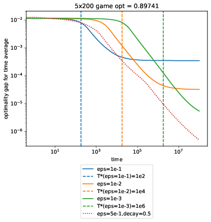
We create game matrices \(M\) of various sizes with entries sampled from a symmetric \(\text{Beta}(0.5, 0.5)\) and compare performance across different \(\epsilon\). opt is the optimal value \(\lambda^* \) in the games below, which we use to plot \(T_* \) for each of our fixed MWUA runs. At each time \(T\), we plot the optimality gap:
\[
\frac{1}{T}\sum_{t}M(\mathcal{D}_t, j_ t) - \lambda^*\,\,.
\]
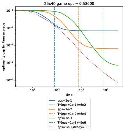

Code @ af5ad62
What’s super curious here is that square-root decay dominates all of the fixed-rate ones, even at their optimal \(T_* \).
Another curiosity is that \(T_*\) looks really off for the final case, where 5 experts square off against an extremely adversarial environment where the column player can choose from 200 columns. To be honest, I don’t know what’s going on here.
Related Work
A weaker version of my requirements above might be methods robust to these concerns:
- Anytime, so a single algorithm works for all \(T\).
- Scale-free, so a single algorithm works for all \(\rho\)
I was able to find these relevant notes, that more or less put all the issues mentioned above to rest:
- Sequential decision-making Lecture 10, Lecture 11, Part 1, Lecture 11, Part 2, Lecture 12
- Elegant AdaHedge, so called because it’s the second version of AdaHedge and it doesn’t use budgeting.
- Steven’s Quora Answer
In short, I want to summarize what I found as the best resources in a field that’s quite saturated: (Freund and Schapire 1999) as the original work and the elegant write-up in Arora’s survey.
Further, Elegant AdaHedge is both anytime and scale-free.
A recent analysis of the Decreasing Hedge, shown above as the square-root decay rate version of hedge helps tidy some things up.
We also have some specializations:
- Constant FTL Regret (FlipFlop, from Elegant AdaHedge paper) - constant-factor performance for the worst case and additive-constant performance compared to the follow-the-leader algorithm.
- Universal Hedge (Decreasing Hedge*) - the “perform within a constant factor of the optimal-constant MWUA for that horizon” guarantee.
- Stochastic Optimality (Decreasing Hedge*) - perform the best when the column player plays randomly (i.e., all experts take losses that are just fixed random variables over time)
*Importantly, decreasing hedge isn’t scale-free, so these claims only hold for \(\rho=1\).