$$ \newcommand{\bsth}{{\boldsymbol\theta}} \newcommand{\nptime}{\textsf{NP}} \newcommand{\ptime}{\textsf{P}} \newcommand{\disteq}{\overset{d}{=}} %linalg \newcommand{\mat}[1]{\begin{pmatrix} #1 \end{pmatrix}} \newcommand{\detmat}[1]{\begin{vmatrix} #1 \end{vmatrix}} \newcommand{\spanb}[1]{\text{span}\{ #1 \}} \DeclareMathOperator{\conv}{conv} % convex hull \DeclareMathOperator{\cone}{cone} \DeclareMathOperator{\vectorize}{vec} \DeclareMathOperator{\matricize}{mat} \DeclareMathOperator{\adj}{adj} \DeclareMathOperator{\diag}{diag} \DeclareMathOperator{\tr}{tr} \DeclareMathOperator{\rank}{rank} \DeclareMathOperator*{\argmin}{argmin} \DeclareMathOperator*{\proj}{proj} % brackets, norms, cardinalities \newcommand{\pa}[1]{ \left({#1}\right) } \newcommand{\ha}[1]{ \left[{#1}\right] } \newcommand{\ca}[1]{ \left\{{#1}\right\} } \newcommand{\inner}[1]{\left\langle #1 \right\rangle} \newcommand{\innercpy}[1]{\inner{ #1, #1 }} \newcommand{\norm}[1]{\left\| #1 \right\|} \newcommand{\abs}[1]{\left|{#1}\right|} \newcommand{\card}[1]{\left\vert{#1}\right\vert} % math vectors \newcommand{\va}{\textbf{a}} \newcommand{\vb}{\textbf{b}} \newcommand{\vc}{\textbf{c}} \newcommand{\vd}{\textbf{d}} \newcommand{\ve}{\textbf{e}} \newcommand{\vf}{\textbf{f}} \newcommand{\vg}{\textbf{g}} \newcommand{\vh}{\textbf{h}} \newcommand{\vi}{\textbf{i}} \newcommand{\vj}{\textbf{j}} \newcommand{\vk}{\textbf{k}} \newcommand{\vl}{\textbf{l}} \newcommand{\vm}{\textbf{m}} \newcommand{\vn}{\textbf{n}} \newcommand{\vo}{\textbf{o}} \newcommand{\vp}{\textbf{p}} \newcommand{\vq}{\textbf{q}} \newcommand{\vr}{\textbf{r}} \newcommand{\vs}{\textbf{s}} \newcommand{\vt}{\textbf{t}} \newcommand{\vu}{\textbf{u}} \newcommand{\vv}{\textbf{v}} \newcommand{\vw}{\textbf{w}} \newcommand{\vx}{\textbf{x}} \newcommand{\vy}{\textbf{y}} \newcommand{\vz}{\textbf{z}} \newcommand{\vzero}{\textbf{0}} \newcommand{\vone}{\textbf{1}} \newcommand{\valpha}{{\boldsymbol\alpha}} \newcommand{\vepsilon}{{\boldsymbol\epsilon}} \newcommand{\vnu}{{\boldsymbol\nu}} \newcommand{\vpi}{{\boldsymbol\pi}} \newcommand{\veta}{{\boldsymbol\eta}} \newcommand{\vsigma}{ {\boldsymbol\sigma}} \newcommand{\vbeta}{ {\boldsymbol\beta}} \newcommand{\vtheta}{ {\boldsymbol\theta}} \newcommand{\vdelta}{ {\boldsymbol\delta}} \newcommand{\vlambda}{ {\boldsymbol\lambda}} \newcommand{\vmu}{ {\boldsymbol\mu}} % common math sets \newcommand{\Z}{\mathbb{Z}} \newcommand{\R}{\mathbb{R}} \newcommand{\C}{\mathbb{C}} \newcommand{\N}{\mathbb{N}} \newcommand{\Q}{\mathbb{Q}} \newcommand{\F}{\mathbb{F}} \newcommand{\T}{\mathbb{T}} % limits \def\sumn{\sum_{n=0}^\infty} \def\limn{\lim_{n\rightarrow\infty}} \def\prodn{\prod_{n=0}^\infty} % mathcal \newcommand{\mcA}{\mathcal{A}} \newcommand{\mcB}{\mathcal{B}} \newcommand{\mcC}{\mathcal{C}} \newcommand{\mcD}{\mathcal{D}} \newcommand{\mcE}{\mathcal{E}} \newcommand{\mcF}{\mathcal{F}} \newcommand{\mcG}{\mathcal{G}} \newcommand{\mcH}{\mathcal{H}} \newcommand{\mcI}{\mathcal{I}} \newcommand{\mcJ}{\mathcal{J}} \newcommand{\mcK}{\mathcal{K}} \newcommand{\mcL}{\mathcal{L}} \newcommand{\mcM}{\mathcal{M}} \newcommand{\mcN}{\mathcal{N}} \newcommand{\mcO}{\mathcal{O}} \newcommand{\mcP}{\mathcal{P}} \newcommand{\mcQ}{\mathcal{Q}} \newcommand{\mcR}{\mathcal{R}} \newcommand{\mcS}{\mathcal{S}} \newcommand{\mcT}{\mathcal{T}} \newcommand{\mcU}{\mathcal{U}} \newcommand{\mcV}{\mathcal{V}} \newcommand{\mcW}{\mathcal{W}} \newcommand{\mcX}{\mathcal{X}} \newcommand{\mcY}{\mathcal{Y}} \newcommand{\mcZ}{\mathcal{Z}} % distribs, probability \newcommand{\disteq}{\overset{d}{=}} \newcommand\independent{\perp \!\!\! \perp} \DeclareMathOperator{\Laplace}{Laplace} \DeclareMathOperator{\Poisson}{Poisson} \DeclareMathOperator{\Exponential}{Exponential} \DeclareMathOperator{\Multinomial}{Multinomial} \DeclareMathOperator{\Bernoulli}{Bernoulli} \DeclareMathOperator{\Categorical}{Categorical} \DeclareMathOperator{\Uniform}{Uniform} \DeclareMathOperator{\Binomial}{Binomial} \DeclareMathOperator{\Hypergeometric}{Hypergeometric} \DeclareMathOperator{\GammaDist}{Gamma} \DeclareMathOperator{\NegativeBinomial}{NegativeBinomial} \DeclareMathOperator\sub{sub} \renewcommand{\d}[1]{\mathop{\mathrm{d} #1 }} \newcommand{\dkl}[2]{\mathop{D_\mathrm{KL}}\left({#1}\;\middle\|\;{#2}\right)} \newcommand{\sg}{\mathop{\mathrm{SG}}} \newcommand{\se}{\mathop{\mathrm{SE}}} %operators \DeclareMathOperator{\power}{{\mathcal{P}}} \DeclareMathOperator{\var}{var} \DeclareMathOperator{\cov}{cov} \DeclareMathOperator\mathProb{\mathbb{P}} \DeclareMathOperator\mathExp{\mathbb{E}} \DeclareMathOperator*\mathExpUnder{\mathbb{E}} \DeclareMathOperator*\fat{fat} \renewcommand{\P}{\mathProb} % need to overwrite stupid paragraph symbol \newcommand{\E}{\mathExp} % need to overwrite stupid paragraph symbol \newcommand{\set}[2]{ \left\{ #1 \,\middle|\, #2 \right\} } \newcommand{\CE}[2]{ \mathExp\left[ #1 \,\middle|\, #2 \right] } \renewcommand{\CP}[2]{ \mathProb\left\{ #1 \,\middle|\, #2 \right\} } $$
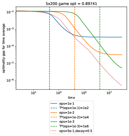
Multiplicative weights is a simple, randomized algorithm for picking an option among \(n\) choices against an adversarial environment.The algorithm has widespread applications, but its analysis frequently introduces a learning rate parameter, \(\epsilon\), which we’ll be trying to get rid of.In this first post, we introduce multiplicative weights and make some practical observations. We follow Arora’s survey for the most part.Problem SettingWe play \(T\) rounds. On the \(t\)-th round, the pla...
Compressed Sensing and SubgaussiansCandes and Tao came up with a broad characterization of compressed sensing solutions a while ago. Partially inspired by a past homework problem, I’d like to explore an area of this setting.This post will dive into the compressed sensing context and then focus on a proof that squared subgaussian random variables are subexponential (the relation between the two will be explained).Compressed SensingFor context, we’re interested in the setting where we observe a...
Subgaussian ConcentrationThis is a quick write-up of a brief conversation I had with Nilesh Tripuraneni and Aditya Guntuboyina a while ago that I thought others might find interesting.This post focuses on the interplay between two types of concentration inequalities. Concentration inequalities usually describe some random quantity \(X\) as a constant \(c\) which it’s frequently near (henceforth, \(c\) will be our stand-in for some constant which possibly changes equation-to-equation). Basical...
Beating TensorFlow Training in-VRAMIn this post, I’d like to introduce a technique that I’ve found helps accelerate mini-batch SGD training in my use case. I suppose this post could also be read as a public grievance directed towards the TensorFlow Dataset API optimizing for the large vision deep learning use-case, but maybe I’m just not hitting the right incantation to get tf.Dataset working (in which case, drop me a line). The solution is to TensorFlow harder anyway, so this shouldn’t reall...
Non-convex First Order MethodsThis is a high-level overview of the methods for first order local improvement optimization methods for non-convex, Lipschitz, (sub)differentiable, and regularized functions with efficient derivatives, with a particular focus on neural networks (NNs).\[\argmin_\vx f(\vx) = \argmin_\vx \frac{1}{n}\sum_{i=1}^nf_i(\vx)+\Omega(\vx)\]Make sure to read the general overview post first. I’d also reiterate as Moritz Hardt has that one should be wary of only looking at con...
Neural Network Optimization MethodsThe goal of this post and its related sub-posts is to explore at a high level how the theoretical guarantees of the various optimization methods interact with non-convex problems in practice, where we don’t really know Lipschitz constants, the validity of the assumptions that these methods make, or appropriate hyperparameters. Obviously, a detailed treatment would require delving into intricacies of cutting-edge research. That’s not the point of this post, w...
Ad Click Prediction: a View from the TrenchesPublished August 2013Paper linkAbstractIntroductionBrief System OverviewProblem StatementFor any given a query, ad, and associated interaction and metadata represented as a real feature vector \(\textbf{x}\in\mathbb{R}^d\), provide an estimate of the probability \(\mathbb{P}(\text{click}(\textbf{x}))\)that the user making the query will click on the ad. Solving this problem has beneficial implications for ad auction pricing in Google’s online adver...