In most data analysis, especially in business contexts, we’re looking for answers about how we can do better. This implies that we’re looking for a change in our actions that will improve some measure of performance.

There’s an abundance of passively collected data from analytics. Why not point fancy algorithms at that?

In this post, I’ll introduce a counterexample showing why we shouldn’t be able to extract such information easily.

Simpson’s Paradox

This has been explained many times, so I’ll be brief. Suppose we’re collecting information about which of two treatments, A or B, better cures kidney stones, regardless of their size.

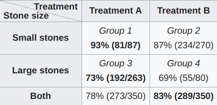
Notice a strange phenomenon: if you know that you have either a small stone or a large stone, you’d want to opt for A, but if you don’t know which of the two stones you have, it looks like B is better, since its cure rate is higher overall.

The counts betray what’s really going on: doctors systematically apply A to harder cases of kidney stones, so even though A performs better on each one, it just has more cases where the average outcome is worse due to their difficulty. Taking the average of the treatment performance across strata resolves the paradox.

Or does it? In this case, we were given the causal knowledge of how doctors apply the treatment to their patients. It is precisely because there’s a causal arrow pointing from kidney stone size to which treatment you’re given that we want to control for kidney stone size.

From an observational perspective, this knowledge doesn’t exist in a set of examples (stone size, treatment, cured or not). As far as that dataset is concerned, stone size could’ve been measured after taking the treatment for a few days, in which case we could still notice the correlations shown in the graph above but wouldn’t want to average in the same way (in particular, treatment A might make the stone bigger before it gets rid of it for some medical reason).

What’s worse, if you don’t see the stone size variable, because you don’t capture it, you’ll make the wrong conclusion about which treatment is more effective.

Knee-jerks

There’s a few reasonable responses from the optimist on this.

1. We capture all relevant variables and know which causes which.
2. We can apply more fanciness.

Note, more fanciness doesn’t just mean you can dump all your variables into an ML model and see what it spits out. There are other pathological cases this approach gives rise to.

But, for the main problem of the above (something called colliders), there are techniques that can identify whether or not they’re present using independence testing. So at first glance the optimist’s approach might be tenable: enough variables, enough smarts to only look at variables with total causal effect on our response, and a sophisticated enough model of the interactions, which we presume fits the situation. We’ll get there, right?

Not quite. An extension of Simpson’s paradox gives us confidence about deeper epistemic uncertainty in causal modelling.

An Infinite Simpson’s Paradox

If we can come up with an example of an infinite Simpson’s paradox, where we have two variables $X,Y$ and they are confounded by $Z_1,Z_2, \cdots$, which go on forever, then regardless of how much data we have, and how many variables we capture, we simply will not be able to tell what the correlation between $X$ and $Y$ is. A “confounder” here is like the kidney stone size—an underlying systematic association that colors what our assessment of $X$’s effect on $Y$ should be.

This gives a precise example to point to. Here’s an instance where you can always have access to as much data instances as you want, as many relevant variables as you want, and all the causal information about those variables, and you’ll still end up with the wrong answer about the average effect of $X$ on $Y$.

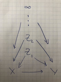
Before jumping into that, let’s be clear about what a diagram like the above means. Every vertex is a random variable. The graph will always be a directed acyclic graph, so there’s an order over the variables sweeping from parents to children, with the eldest parents having no parents themselves (they’re the roots, in this case $Z_j$).

If you define the marginal distribution $p(z_j)$ of the roots and the conditional probabilities of every child given their parents, then you’ve defined the full joint distribution of every variable in the graph. For example, for the graph $\mcG$ below,

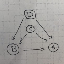
it’s easy to convince ourselves that for the parent operation $\mathrm{Pa}$ that returns a node’s parents, \[ p(a, b, c, d)=\prod_{v\in\mcG}p(v|\mathrm{Pa}(v))=p(c)p(d)p(b|c, d)p(a|b, c, d)\,\,, \] but what does this mean when we have infinitely many variables as shown in the previous diagram?