This is Problem 9.11 in Elements of Causal Inference.

_Construct a single Bayesian network on binary $X,Y$ and variables $\{Z_j\}_{j=1}^\infty$ where the difference in conditional expectation,

\[\begin{align} \Delta_j(\vz_{\le j}) &=\\ & \CE{Y}{X=1, Z_{\le j}=\vz_{\le j}}-\\ & \CE{Y}{X=0, Z_{\le j}=\vz_{\le j}}\,\,, \end{align}\]

satisfies $\DeclareMathOperator\sgn{sgn}\sgn \Delta_j=(-1)^{j}$ and $\abs{\Delta_j}\ge \epsilon_j$ for some fixed $\epsilon_j>0$. $\Delta_0$ is unconstrained._

Proof overview

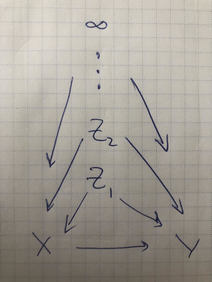
We will do this by induction, constructing a sequence of Bayes nets $\mcC_d$ for $d\in\N$ with variables $X,Y,Z_1,\cdots,Z_d$, such that $\mcC_d\subset\mcC_{d+1}$, in a strict sense. In particular, our nets will be nested so that they have the same structure on common variables. This means that for their entailed respective joints $p_d,p_{d+1}$, \[ p_d(x, y, z_{1:d})=\int\d{z_{d+1}}p_{d+1}(x, y, z_{1:d+1})\,\,. \]

Intuitively, this seems to lead us to a limiting structure $\mcC_\infty$ over the infinite set of nodes, but it’s not clear that this necessarily exists. Our ability to generate larger probability spaces by adding independent variables doesn’t help here, since those are finite tools.

For simplicity, we’ll construct $X$ such that its marginal has mass $b(x)=0.5$ for $x=0,1$. We’ll also take $Z_j$ to be binary. Nonetheless, even in this simple setting, the set of realizations of $\{Z_j\}_{j=1}^\infty$ is uncountable, $2^\N$. Assigning probabilities to every subset of this set isn’t easy.

So first we’ll have to tackle well-definedness. What does $\mcC_\infty$ even mean, mathematically? Equiped with this, we can specify more details about the specific $\mcC_\infty$ we want to have that’ll satisfy properties about $\Delta_j$.

Well-definedness of $\mcC_\infty$

Suppose that we have open unit interval-valued functions $\alpha_x,\beta_x$ for $x\in\{0,1\}$ on binary strings that satsify, for any $j\in\N$ and binary $j$-length string $\vz$, that \[ \beta_x(\vz)=(1-\alpha_x(\vz))\beta_i(\vz:0)+\alpha_x(\vz)\beta_x(\vz:1)\,\,, \] where $\vz:i$ is the concatenation operation (at the end). We construct an object $\mcC_\infty$ defined by finite kernels $p(x|\vz_J),p(y|x,\vz_J),p(\vz_J)$ (that is, for any $J\subset \N$, $\mcC_\infty$ provides us with these functions) that induce a joint distribution over $(X, Y, Z_J)$. Moreover, there exists unique law $\P$ Markov wrt $\mcC_\infty$ (it is consistent with the kernels), which adheres to the following equality over binary strings $\vz$ of length $j$ with $Z=(Z_1,\cdots, Z_j)$:

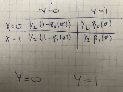
\[\begin{align} \beta_i(\vz)&=\CP{Y=1}{X=i,Z=\vz}\\ \alpha_i(\vz)&=\CP{Z_j=1}{X=i,Z=\vz}\,\,. \end{align}\]

Proof

The proof amounts to specifying Markov kernels inductively in a way that respects the invariant promised, and then applying the Kolmogorov extension theorem. While this would be the way to formally go about it, an inverse order, starting from Kolmogorov, is more illustritive.

The theorem states that given joint distributions $p_N$ over arbitrary finite tuples $N\subset \{X,Y,Z_1, Z_2,\cdots\}$ which match the consistency property $p_K=\int\d{\vv}p_N$, where $\vv$ is the realization of variables $N\setminus K$ for $K\subset N$, there exists a unique law $\P$ matching all the joint distributions on all tuples (even infinite ones). That is, you need be consistent under marginalization.

Before diving in, we make a few simplifications.

1. Since the variables are all binary it’s easy enough to make sure all our kernels are valid conditional probability distributions; just specify a valid probability for one of the outcomes, the other being the complement.
2. We’ll focus only on kernels $p(z_j)$, $p(x|\vz_{\le j})$, and $p(y|x, \vz_{\le j})$ for $j\in\N$. It’s easy enough to derive the other ones; for any finite $J\subset \N$, with $m=\max J$, just let \[ p(x|\vz_J)=\int\d{\vz_{[m]\setminus J}}p(x|\vz_{\le m})p(\vz_{[m]\setminus J})\,\,, \] and analogously for $p(y|x, \vz_{\le j})$. Thanks to independence structure, $p(\vz_J)=\prod_{j\in J}p(z_j)$.

Extension

This simplification in (2) means when checking the Kolmogorov extension condition, we needn’t worry about differences in $N$ and $K$ by $Z_j$ nodes.

Consider tuples $K\subset N$ over our variables from $\mcC_\infty$, and denote their intersections with $\{Z_j\}_{j\in\N}$ as $Z_{J_K},Z_{J_N}$. Letting $m=\max J_N$,

\[\begin{align} p_K(x, y, \vz_{J_K})&= p_K(y|x, \vz_{J_K})p_K(x|\vz_{J_K})p(\vz_{J_K})\\ &=\int\d{\vz_{[m]\setminus J_K}}p(y|x, \vz_{\le m})p(x|\vz_{\le m})p(\vz_{\le m})\\ &=\int\d{\vz_{J_N\setminus J_K}}\int\d{\vz_{[m]\setminus J_N}}p(y|x, \vz_{\le m})p(x|\vz_{\le m})p(\vz_{\le m})\\ &=\int\d{\vz_{J_N\setminus J_K}}p_N(y|x, \vz_{J_N})p_N(x|\vz_{J_N})p_N(\vz_{J_N})\\ &=\int\d{\vz_{J_N\setminus J_K}}p_N(x, y, \vz_{J_N})\,\,. \end{align}\]

The subscripts are important here. Of course, $p_K(\vz_L)=p_N(\vz_L)=p(\vz_L)=\prod_{j\in L}p(z_j)$ for any $L\subset K\subset N$ by independence and kernel specification. Otherwise, the steps above rely on joint decomposition, then simplification (2) applied to $K$, Fubini, then simplification (2) applied to $N$ now in reverse, and finally joint distribution composition.

The above presumes $X,Y\in K$, but it’s clear that we can simply add in the corresponding integrals on the right hand side to recover them if they’re in $N$ after performing the steps above.

The above finishes our use of the extension theorem, relying only on the fact that we constructed valid Markov kernels to provde us a law $\P$ consistent with them. But to actually apply this reasoning, we have to explicitly construct these kernels, which we’ll do with the help of simplification (1).

Kernel Specification

We show that there exist marginals $p(z_j)$ such that $p(x)$ is the Bernoulli pmf $b(x)$ and $p(z_j|x,\vz_{<j})$ is defined by $\alpha_x(\vz_{<j})$. In particular, we first inductively define $p(x|\vz_{\le j})$ and $p(z_j)$ simultaneously. For $j=0$ set $p(x)=b(x)$. Then for $j>0$ define \[ p(Z_j=1)=\int\d{(x,\vz_{<j})}\alpha_x(\vz_{<j})p(x|\vz_{<j})p(\vz_{<j})\,\,, \] which for $j=1$ simplifies to $p(Z_1=1)=\int \d{x}p(x)\alpha_x(\emptyset)=b(0)\alpha_0(\emptyset)+b(1)\alpha_1(\emptyset)$, and then use that to define \[ p(X=1|\vz_{\le j})=\frac{\alpha_x(\vz_{\le j})p(x|\vz_{<j})}{p(z_j)}\,\,, \] which induces $p(x|\vz_{\le j})$. For the case of $j=1$ the above centered equation simplifies to $\alpha_x(z_1)b(x)/p(z_1)$. It is evident from Bayes’ rule applied to $p(x|z_j,\vz_{< j})$ that this is the unique distribution $p(x|\vz_{\le j})$ matching the semantic constraint on $\alpha_x$, assuming $Z_j$ are independent.

Uniqueness of $p(x|\vz_{\le j})$ follows inductively, as does $\int \d{\vz_{\le m}}p(x|\vz_{\le m})p(\vz_{\le m})=b(x)$.

While above we could construct conditional pmfs and marginals pmfs to suit our needs, where they formed valid measures simply by construction (i.e., specifying any open unit interval valued $\alpha$ constructs valid pmfs above), we must now use our assumption to validate that the free function $\beta$ induces a valid measure on $Y$.

It must be the case that for any kernel we define that for all $j\in \N$, \[ p(y|x, \vz_{\le j})=\int\d{z_{j+1}}p(z_{j+1}|x, \vz_{\le j})p(y|x, \vz_{\le j+1})\,\,, \] which by the assumption $\beta_x(\vz)=(1-\alpha_x(\vz))\beta_i(\vz:0)+\alpha_x(\vz)\beta_x(\vz:1)$ holds precisely when \[ p(Y=1|x, \vz_{\le j})=\beta_x(\vz_{\le j})\,\,, \] by our definition of $p(z_{j+1})$ above. Then such a specification of kernels is valid.

Configuring $\Delta_j$

Having done all the work in constructing $\mcC_\infty$, we now just need to specify $\alpha, \beta$ meeting our constraints.

To do this, it’s helpful to work through some examples. We first note a simple equality, which is \[ \Delta_d(\vz)=\beta_1(\vz)-\beta_0(\vz)\,\,. \]

For $d=0$, we can just take $\beta_0(\emptyset)=\beta_1(\emptyset)=0.5$

For $d=1$, we introduce $Z_1$. Notice we now are bound to our constraints,

\[\begin{align} \beta_0(\emptyset)&=(1-\alpha_0(\emptyset))\beta_i(0)+\alpha_0(\emptyset)\beta_0(1)\\ \beta_1(\emptyset)&=(1-\alpha_1(\emptyset))\beta_i(0)+\alpha_1(\emptyset)\beta_1(1)\,\,. \end{align}\]

At the same time, we’re looking to find settings such that $\forall z,\,\,\beta_1(z)-\beta_0(z)\le -\epsilon$.

Luckily, our constraints amount to convexity constraints; algebraicly, this means that $\beta_0(0),\beta_0(1)$ must be on either side of $\beta_0(\emptyset)$ and similarly for $\beta_1(\emptyset)$. At the same time, we’d like to make sure that $\beta_0(1)-\beta_1(1)\ge \epsilon_1$. This works out! See the picture below, which sets \[ (\beta_1(0), \beta_0(0),\beta_1(1),\beta_0(1))=0.5+\pa{-2\epsilon_1,-\epsilon_1,\epsilon_1,2\epsilon_1}\,\,. \]

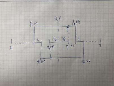
Then, choice of $\alpha_i(\emptyset)$ meets the constraints.

For the recursive case, recall we need \[ \beta_x(\vz)=(1-\alpha_x(\vz))\beta_x(\vz:0)+\alpha_x(\vz)\beta_x(\vz:1)\,\,, \] so we’ll choose $\beta_x(\vz:1)>\beta_x(\vz)>\beta_x(\vz:0)$, which always admits solutions on the open unit interval, but to ensure that $\beta_1(\vz:z_j)-\beta_0(\vz:z_j)=(-1)^{j}\epsilon_j$, we need another construction similar to the above with the number line. Here’s the next step.

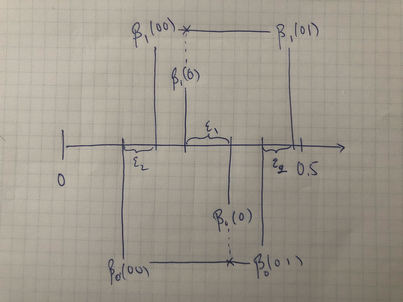
Where we can frame the above recursively. Suppose $m$ is the minimum distance from $\beta_1(\vz),\beta_0(\vz)$ to $0,1$. Without loss of generality assume the parity of $\vz$ is such that we’re interested in having $\beta_1(\vz:z_j)>\beta_0(\vz:z_j)$, which implies by parity as well that in the previous step $\beta_1(\vz)\le \beta_0(\vz)$.

Then for $j=\card{\vz}+1$ set \[ \mat{\beta_0(\vz:0)\\ \beta_1(\vz:0)\\\beta_0(\vz:1)\\\beta_1(\vz:1) }= \mat{\beta_1(\vz)-\frac{m+\epsilon_{j}}{2} \\ \beta_1(\vz)-\frac{m-\epsilon_{j}}{2} \\ \beta_0(\vz)+\frac{m-\epsilon_{j}}{2} \\ \beta_0(\vz)+\frac{m+\epsilon_{j}}{2} }\,\,. \]

This recursion keeps the equations solvable, and by choice of $\epsilon_{j}$ sufficiently small all quantities are within $(0,1)$.