One neat takeaway from the previous post was really around the structure of what we were doing.
What did it take for the infinite DAG we were building to become a valid probability distribution?
We can throw some things out there that were necessary for its construction.
- The infinite graph needed to be a DAG
- We needed inductive “construction rules” $\alpha,\beta$ where we could derive conditional kernels from a finite subset of infinite parents to a larger subset of the infinite parents.
- The construction rules need to be internally consistent so as to satisfy Kolmogorov’s extension theorem.
Plate Notation
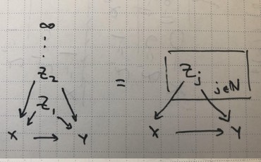
We’ll borrow plate notation from graphical models literature, where you can generate variable-size models by taking the union of the graphs for each index in the plate.
Examples
The first two rules (DAG, construction rules) seem intuitive. Further, from a probibalist’s perspective, rule (3) is just as self-evident. The rule is exactly the Kolmogorov consistency condition: we’ll admit all construction rules that generate joints which are externally consistent.
But this doesn’t quite touch on some interesting interaction with structure. For instance, we have our familiar infinite Simpson’s paradox diagram.
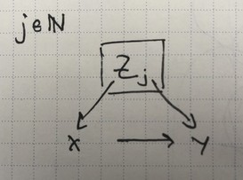
We have our construction rules, which correspond roughly to the two points where an arrow crosses a plate, at $X\leftarrow Z_j$ and $Z_j\rightarrow Y$.
\[\begin{align} \beta_i(\vz)&=\CP{Y=1}{X=i,Z=\vz}\\ \alpha_i(\vz)&=\CP{Z_j=1}{X=i,Z=\vz}\,\,. \end{align}\]Next, the consistency rule $\beta_x(\vz)=(1-\alpha_x(\vz))\beta_i(\vz:0)+\alpha_x(\vz)\beta_x(\vz:1)$ seems to correspond to the (undirected) loop formed by $X,Y,Z_j$.
We go on. Here’s the double infinite Simpson’s paradox diagram.

A few things emerge. If we leave the arrow $A\leftarrow B$ in there, it’s clear we have two independent Simpson’s paradox structures. The undirected loops birth two consistency rules, and we expect four builder rules for each plate/arrow crossing.
If we remove the arrow $A\leftarrow B$, the consistency rule goes away: you just need to specify the builder rules between $Z$ and each of $A,B$ individually.
Visually, a few other things become clear. As far as we’re concerned, chains aren’t that important. If we had $X\rightarrow Q\rightarrow Y$ in the above diagrams instead of $X\rightarrow Y$, there would be an extra few terms but we’d only have once consistency rule, still.
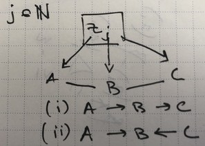
Let’s keep going. Here’s where things get spicy. The overlapping loops diagram has two cases, (i) with one direction of arrows and (ii) with a collider.
Having a chain in plate don’t seem interesting.
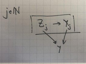
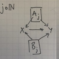
Finally, we can mix things up with another plate, here with two loops with a shared regular edge.
Open Questions
What’s the role of builder rule parameterization? In the infinite Simpson’s paradox, I specifically chose
\[\begin{align} \beta_i(\vz)&=\CP{Y=1}{X=i,Z=\vz}\\ \alpha_i(\vz)&=\CP{Z_j=1}{X=i,Z=\vz}\,\,. \end{align}\]because $\beta_i$ was a useful parameterization for computing the difference $\Delta_j(\vz)$. Perhaps
\[\begin{align} \beta_{y}(\vz)&=\CP{Z_j=1}{Y=y,Z=\vz}\\ \alpha_x(\vz)&=\CP{Z_j=1}{X=x,Z=\vz} \end{align}\]is more natural as the set of builder rules. What constraint does this require?
It seems like we get consistency constraints for every junction that has an “infinite probability flow”. That is, if there’s two directed paths like $Z_j\rightarrow X\rightarrow Y$ and $Z_j\rightarrow Y$ with a source that’s an infinite plate and the same sink, then we’ll expect a consistency rule for each path. The paths can have different infinite sources, such as shared regular edge diagrma’s junction for $A_j,B_j\rightarrow X$.
In the case of an overlapping loop (ii), we have three directed paths meeting at junction $B$, so we have a consistency rule over three builder rules simultaneously.
There’s bound to be some very pretty, minimal, category-theoretic way of expressing Kolmogorov-extensible DAGs. This is useful because it gives us a natural parameterization of such conditional structures, with the minimal amount of constraints on conditional probability kernels.