Step aside, map reduce. In this post, I’ll introduce a single-machine utility for parallel processing that significantly improves upon the typical map-reduce approach. When dealing with GB-to-TB size datasets, using a large multiprocessing machine should be enough for fast computation, but performance falls short of expectations due to naive reduce implementations.

Let’s take the canonical map reduce example, word count, where our goal is to take a corpus of text and construct a map from words to the number of times they appear in the corpus. We’ll be working with a 16-core machine throughout this post.

Let’s grab 1GB of English wikipedia for a running example and do some lightweight cleaning.

curl -o enwik9.bz2 https://cs.fit.edu/~mmahoney/compression/enwik9.bz2
bunzip2 enwik9.bz2
tr '[:upper:]' '[:lower:]' enwik9 | tr -c '[:alnum:]- \n' ' ' > enwik9.clean
rm enwik9
tail -1 enwik9.clean  | tr -s " "; echo
# breathing high-pressure oxygen for long periods can causes oxygen toxicity one of the side effects 

Let’s do a typical map-reduce with spark to get the top words.

pyspark
...
>>> from operator import add
>>> from collections import Counter
>>> ctr = spark.read.text('enwik9.clean')\
...   .rdd.mapPartitions(lambda rs: [
...     Counter(w for r in rs
...       for w in r[0].split(' ') if w)])\
...   .reduce(add) 
>>> ctr.most_common(5)
[('the', 7797642), ('of', 4855049), ('and', 3059322), ('in', 2621192), ('a', 2332364)]

This takes about 64 sec. If we track cpu and memory utilization during the above run, we’ll notice something strange:

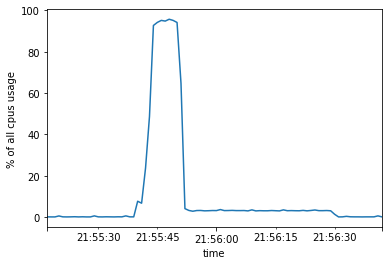
Towards the end of the computation, we have long stretches of almost serial code. Why is that? The problem is visible from the computation graph of this map reduce job.

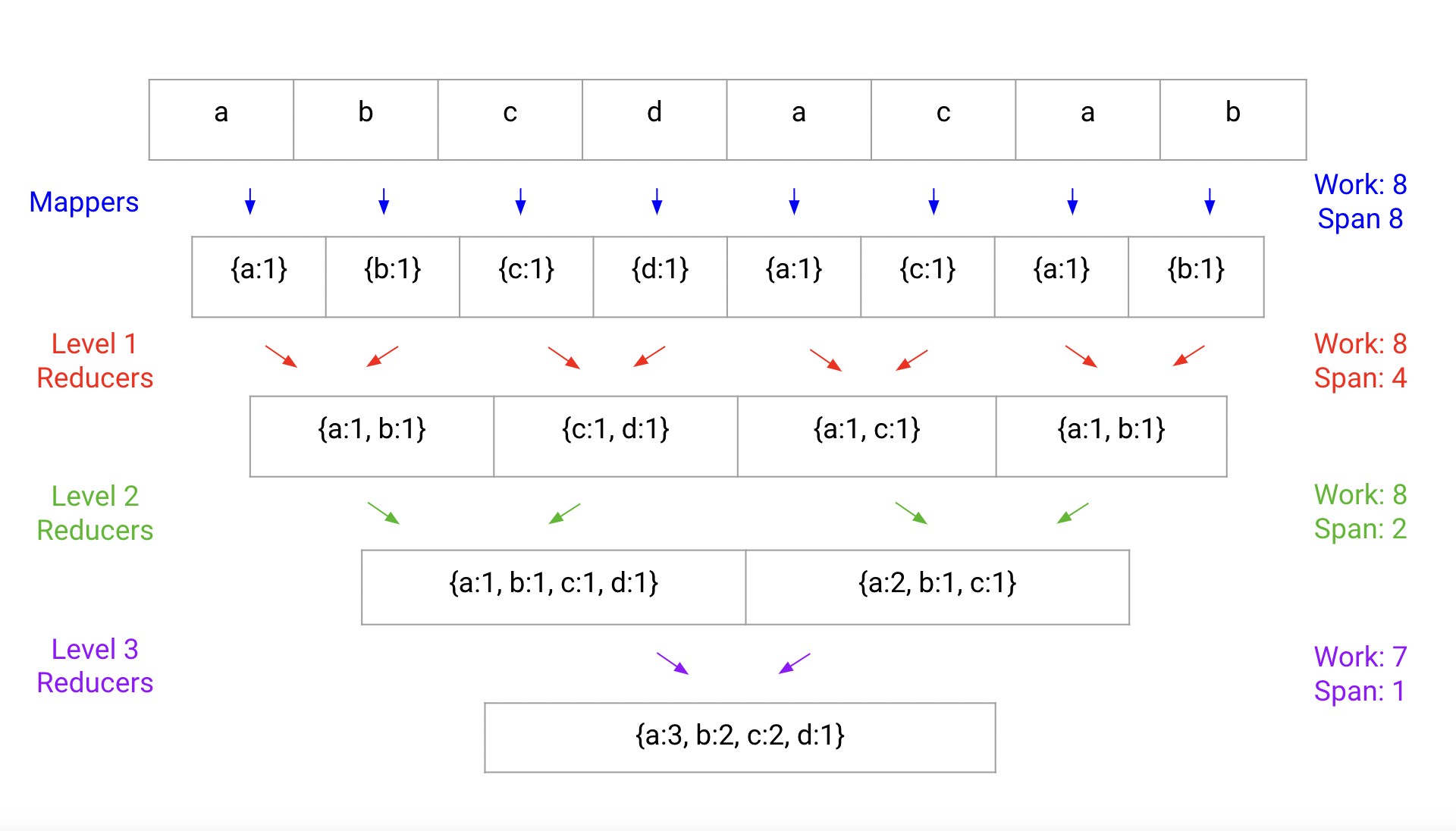
As we go down the computation, we distill words into word-count pairs. This does O(corpus size) work and can be infinitely parallelized. But in the reduce steps we need to combine many small hashmaps together to retrieve the final hashmap. At each level, we combine pairs of hashmaps. The total work done across all combination step is O(num unique words), yet the number of hashmap pairs to combine drops to 1. So we’re stuck waiting at the end for a single worker combining the final map.

What can we do to fix the situation? The problem stems from the fact that our final output—a map from words to counts—is much larger than tolerable to process serially. So, no matter what, an interface such as map reduce which returns a “serial object” such as a regular, single-threaded hashmap is doomed to require the large O(num unique words) processing step on one thread at some point.

Sure, we could look into lockfree or multi-threaded hashmaps, assuming a shared-memory system, but per Joe Hellerstein’s “swim-lane” intuition, it’d be preferable to instead have a framework which keeps data local to a single CPU’s cache as much as possible (this preference is also amenable to distributed computation later, unlike shared-memory approaches).

Map reduce relies on the following abstractions, which naturally lead to a single output “serial object” \(U\) from a collection of inputs of type \(X\):

where \(\mathrm{reduce}\) is a commutative, associative operation. Instead, an API like

ends up being very natural in a Unix setting, and aside from purity of the \(\mathrm{flatmap},\mathrm{fold}\) functions has no requirements. Schematically, it looks like this:

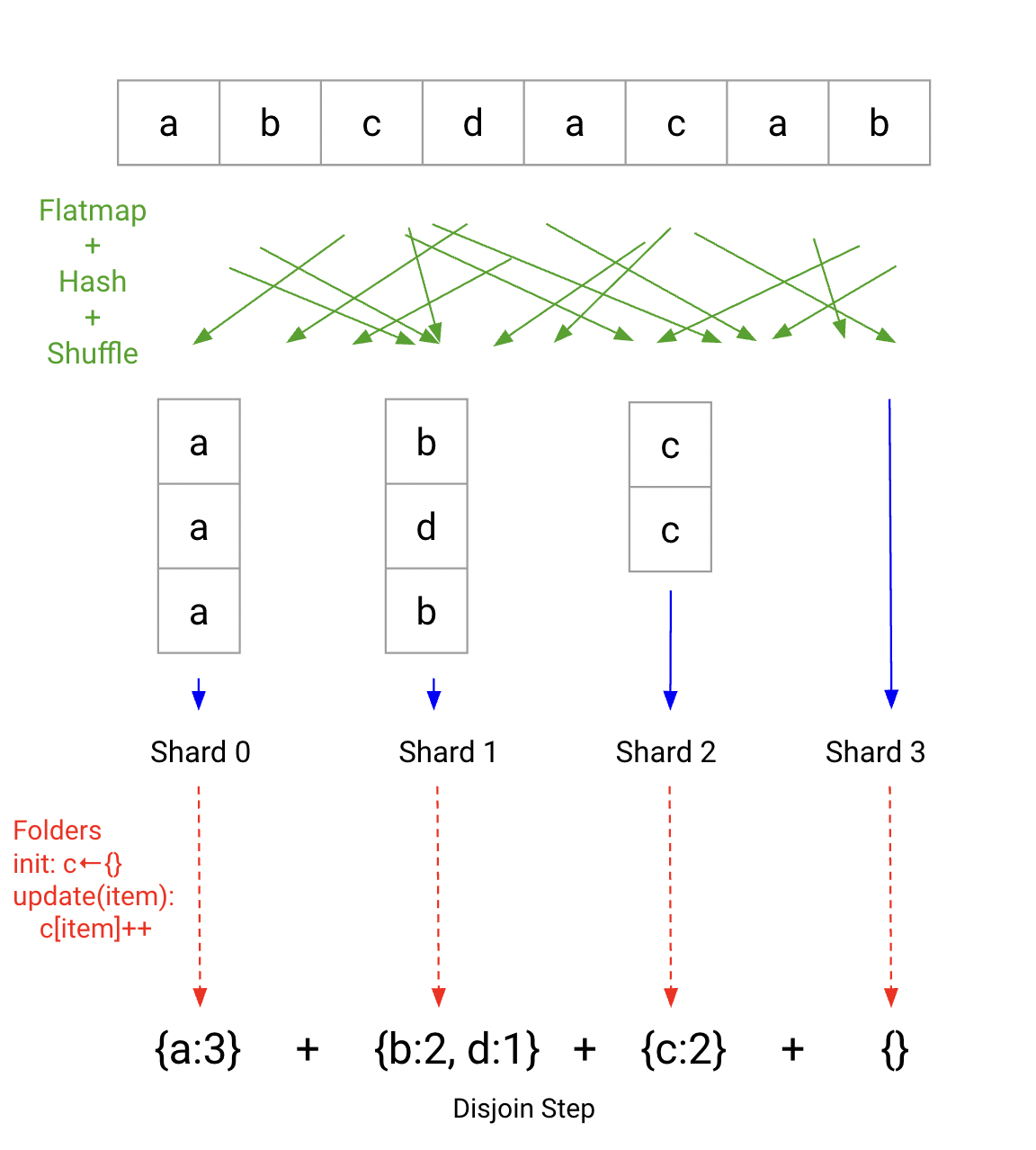
Note, this requires actually changing what our result is. We’re no longer offering a serial hashmap of our keys, but rather a disjunction over disjoint hashmaps. This requires no additional merges, thanks to disjointness.

The advantage of this approach over map reduce for keyed inputs is that (1) there are no serial reduce steps, (2) all the computational steps can be made online and (3) memory usage is bounded, unlike the tree reduce approach, where in principle all keys could be replicated across multiple transient unreduced maps.

I implemented a version of the above for a unix-like text stream interface. slb (for “sharded load balance”) essentially works like parallel --pipe --roundrobin would, splitting its input based on hash, and maintaining parallel independent mapper processes and folding processes which are to emit lines at the end of computation. The disjunction step here is just line concatenation (where the output lines for wordcount are key-value pairs).

Let’s revisit our wordcount benchmark with our new approach.

/usr/bin/time -f "%e sec" target/release/slb \
  --mapper 'tr " " "\n" | rg -v "^$"' \
  --folder "awk '{a[\$0]++}END{for(k in a)print k,a[k]}'" \
  --infile enwik9.clean \
  --outprefix wikslb.
# 6.20 sec
cat wikslb.* | sort --parallel=$(nproc) -k2nr -k1 | head -5
# the 7797642
# of 4855049
# and 3059322
# in 2621192
# a 2332364

Much better! The flatmap operation tr " " "\n" | rg -v "^$", which puts every word on its own line, is a natural Unix line streaming operation. The folder, awk '{a[$0]++}END{for(k in a)print k,a[k]}' statefully tracks a simple keyed counter. This makes slb a fitting primitive for parallelizing keyed aggregations in the Unix way, which is convenient for ML use cases such as:

• feature frequency counting
• distinct feature value aggregation and counting

There’s all sorts of interesting extensions to be made for slb; check out the repo for details and examples.

• How could we support multiple input files?
• Do buffer and queue sizes affect performance? Can they be autotuned?
• Are stragglers causing problems?

Illustrations provided by Olivia Wynkoop.

P.S. Nowadays, Spark has a more advanced API which can look at the full AST of our parallel computation:

pyspark
...
>>> from pyspark.sql.functions import split, col, explode
>>> ctr = spark.read.text('enwik9.clean')\
...    .select(explode(split(col('value'), '\s+')).alias('word')) \
...    .where(col('word') != '') \
...    .groupby('word') \
...    .count() \
...    .collect()
>>> ctr.sort(key=lambda r: r["count"])
>>> ctr[-5:]
[Row(word='a', count=2332364), Row(word='in', count=2621192), Row(word='and', count=3059322), Row(word='of', count=4855049), Row(word='the', count=7797642)]

The groupby portion now runs in 34 sec. As we can see, we have much higher utilization too:

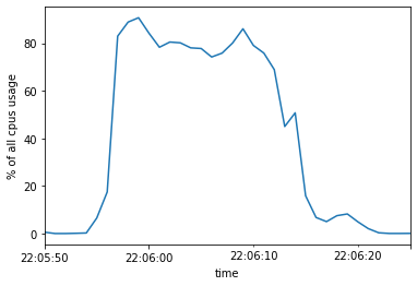
However, this is still slower than using the Unix utilities with slb.