Articles by category: parallel

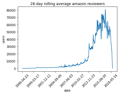
To show off a recent command line tool for sketching, dsrs, let’s plot the rolling 28-day average daily count of active reviewers on Amazon.The raw data here is item,user,rating,timestamp so this would map to a sophisticated GROUP BY with a COUNT DISTINCT over 28-day windows in SQL. But since the data’s only available as CSV, how can we get to the same answer? If we’re just interested in an approximate solution, can we do this without using a bunch of memory or custom (shuffle-inducing…) slid... Read More

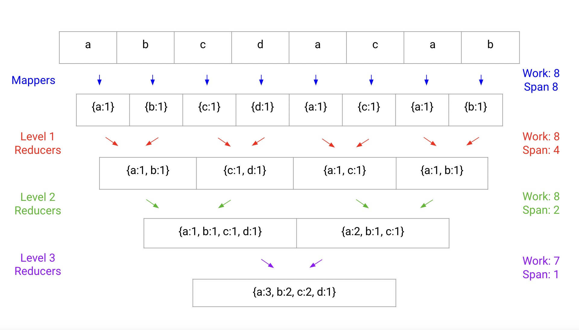
Step aside, map reduce. In this post, I’ll introduce a single-machine utility for parallel processing that significantly improves upon the typical map-reduce approach. When dealing with GB-to-TB size datasets, using a large multiprocessing machine should be enough for fast computation, but performance falls short of expectations due to naive reduce implementations.Let’s take the canonical map reduce example, word count, where our goal is to take a corpus of text and construct a map from words... Read More

Markov Chain Monte Carlo methods (MCMC) are, functionally, very cool: they enable us to convert a specification of a probability distribution from a likelihood \(\ell\) into samples from that likelihood. The main downside is that they’re very slow. That’s why lots of effort has been invested in data-parallel MCMC (e.g., EPMCMC). This blog post takes a look at a specialized MCMC sampler which is transition-parallel, for a simple distribution: Given a fixed, simple, large graph \(G=(V,E)\) on ... Read More

FAISS, Part 1FAISS is a powerful GPU-accelerated library for similarity search. It’s available under MIT on GitHub. Even though the paper came out in 2017, and, under some interpretations, the library lost its SOTA title, when it comes to a practical concerns: the library is actively maintained and cleanly written. it’s still extremely competitive by any metric, enough so that the bottleneck for your application won’t likely be in FAISS anyway. if you bug me enough, I may fix my one-line E... Read More

FAISS, Part 2I’ve previously motivated why nearest-neighbor search is important. Now we’ll look at how FAISS solves this problem.Recall that you have a set of database vectors \(\{\textbf{y}_i\}_{i=0}^\ell\), each in \(\mathbb{R}^d\). You can do some prep work to create an index. Then at runtime I ask for the \(k\) closest vectors in \(L^2\) distance.Formally, we want the set \(L=\text{$k$-argmin}_i\norm{\textbf{x}-\textbf{y}_i}\) given \(\textbf{x}\).The main paper contributions in this rega... Read More

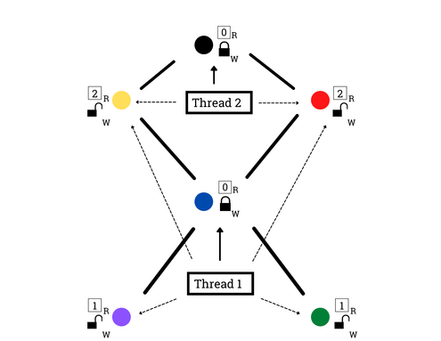
The Semaphore BarrierThis is the answer post to the question posed here.A Useful FormalismReasoning about parallel systems is tough, so to make sure that our solution is correct we’ll have to introduce a formalism for parallel execution.The notion is the following. Given some instructions for threads \(\{t_i\}_{i=0}^{n-1}\), we expect each thread’s individual instructions to execute in sequence, but instructions between threads can be interleaved arbitrarily.In our simplified execution model ... Read More

The Semaphore BarrierI wanted to share an interview question I came up with. The idea came from my operating and distributed systems classes, where we were expected to implement synchronization primitives and reason about concurrency, respectively.Synchronization primitives can be used to coordinate across multiple threads working on a task in parallel.Most primitives can be implemented through the use of a condition variable and lock, but I was wondering about implementing other primitives i... Read More

MapReduce: Simplified Data Processing on Large ClustersPublished December 2004Paper linkAbstractMapReduce offers an abstraction for large-scale computation by managing the scheduling, distribution, parallelism, partitioning, communication, and reliability in the same way to applications adhering to a template for execution.IntroductionProgramming ModelMR offers the application-level programmer two operations through which to express their large-scale computation.Note: the types I offer here a... Read More

Ad Click Prediction: a View from the TrenchesPublished August 2013Paper linkAbstractIntroductionBrief System OverviewProblem StatementFor any given a query, ad, and associated interaction and metadata represented as a real feature vector \(\textbf{x}\in\mathbb{R}^d\), provide an estimate of the probability \(\mathbb{P}(\text{click}(\textbf{x}))\)that the user making the query will click on the ad. Solving this problem has beneficial implications for ad auction pricing in Google’s online adver... Read More

Ligra: A Lightweight Graph Processing Framework for Shared MemoryPublished February 2013Paper linkAbstractLigra graph processing goals: Single machine, shared memory, multicore Lightweight BFS Mapping over vertex subsets Mapping over edge subsets Adapt to varying vertex degreesIntroductionMotivation for Single Machine FrameworkLower communication cost allows for performance benefits.Current demands do not necessitate the distributed computation framework previous implementations provide... Read More