Ad Click Prediction: a View from the Trenches
Published August 2013
Abstract
Introduction
Brief System Overview
Problem Statement
For any given a query, ad, and associated interaction and metadata represented as a real feature vector \(\textbf{x}\in\mathbb{R}^d\), provide an estimate of the probability \(\mathbb{P}(\text{click}(\textbf{x}))\)that the user making the query will click on the ad. Solving this problem has beneficial implications for ad auction pricing in Google’s online advertising business.
Further problem details:
- \(d\) is in the billions - naive dense representation of one data point would take GBs!
- Features are “extremely sparse”
- Serving must happen quickly, at a rate of billions of predictions per day. Though never mentioned explicitly in the paper, I’m assuming the training rate (dependent on the actual number of ads shown, not considered) is thus a small fraction of this but still considerable.
Given sparsity level and scalability requirements, online regularized logistic regression seems to be the way to go. How do we build a holistic machine learning solution for it?
Vowpal Wabbit was developed a few years before a solution to these kinds of problems, but handled several orders of magnitudes less (its dictionary size is \(2^{18}\) by default).
Note: in the discussion below we’ll be assuming most of the features are categorical variables, represented as indicators with strings as the feature names.
Online Learning and Sparsity
Preamble
The paper uses the compressed notation for the sum of the \(i\)-th gradients: \(\textbf{g}_{1:t}=\sum_{i=1}^t\textbf{g}_i\), where the gradient is computed from the logistic loss of the \(t\)-th example \(\textbf{x}_t\), given for the prediction \(y_t\in{0,1}\) given the current weight \(\textbf{w}_t\).
Predictions are made according to the sigmoid, where \(p_t=\sigma(\textbf{w}_t\cdot\textbf{x}_t)\) and \(\sigma(a)=(1+\exp(-a))^{-1}\). Loss is: \[ \ell_t(\textbf{w}_t)=-y_t\log p_t-(1-y_t)\log(1-p_t) \]
Its unregularized gradient is: \[ \nabla \ell_t(\textbf{w}_t)=(p_t-y_t)\textbf{x}_t \]
The \(i\)-th element of a vector \(\textbf{v}\) will be be given by the unbolded letter \(v_i\).
Sparsity
Completely-0 sparsity is essential because of the large number of features (thus susceptibility to overfitting) and because a sparse coefficient representation scales memory consumption with non-zeros.
\(L_1\) penalty subgradient approaches alone aren’t good enough. \(L_1\) won’t actively discourage zeros like \(L_2\) does, but while usually considered sparsity-inducing it’s more accurately sparsity ambivalent: as a weight gets smaller, its penalty follows linearly.
Some alternative approaches have more active sparsity induction: FOBOS and RDA. I have no idea what they are, but apparently FTRL-Proximal is better anyway (see Table 1 in the paper).
FTRL-Proximal
FTRL-Proximal is an \(L_1\)-regularized version of the Follow The Regularized Leader. FTRL is a core online learning algorithm. It improves upon a naive one, called Follow The Leader, or FTL, where the best coefficients in hindsight \(\textbf{w}_{t}^*\) are chosen for the next step:
\[ \textbf{w}_{t+1}=\textbf{w}_t^*=\underset{\textbf{w}}{\mathrm{argmin}}\sum_{i=1}^t\ell_i(\textbf{w}) \]
Of course, this strategy can be pathologically unstable; consider the expert problem where two experts are alternatingly correct, but the one you choose first is wrong - then you’d be switching to the wrong expert each time.
Borrowing Prof. Hazan’s notation \(\nabla_i=\nabla\ell_i(\textbf{w}_i)\), the regret contribution for the \(i\)-th guess at time \(t\) is \(\ell_i(\textbf{w}_i)-\ell_i(\textbf{w}_{t}^*)\).
This is bounded above by \(\nabla_t^T (\textbf{w}_i-\textbf{w}_{t}^*)\) assuming convexity of each \(\ell_i\).
If we look at the related equation for the upper bound of the total regret up to time \(t\):
\[ \text{regret}_t\le \sum_{i=1}^t \nabla_t^T (\textbf{w}_i-\textbf{w}_{t}^*) \]
We see that FTL is equivalent to optimizing that bound for the previous iterations. In fact, optimizing this bound is all we can do: we don’t know each \(\ell_i\) ahead of time, so we solve the generic bound for any differentiable convex loss, only using the observed gradient \(\nabla_i\), instead. But, as the example above mentioned, it performs poorly because it can be unstable. FTRL introduces some notion of stability to the algorithm by changing the optimization goal to:
\[ \textbf{w}_{t+1}=\underset{\textbf{w}}{\mathrm{argmin}} \sum_{i=1}^t \eta_t\nabla_t^T (\textbf{w}_i-\textbf{w}_{t}^*) +R(\textbf{w}) \]
The \(\eta_t\) factors control how much the regularization function affects the next guess. By observing that \(\textbf{w}_{t}^*\) is a constant, and choosing \(R\) appropriately, we have the new convex update for a particular FTRL algorithm, FTRL-Proximal:
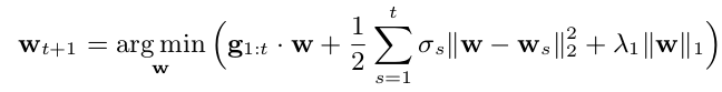
We inductively define \(\sigma_{1:i}=\eta_{i}^{-1}\) (for \(\eta_t=O(t^{-1})\) this is eventually monotonically nonincreasing) and let \(\textbf{g}_i=\nabla_i\). As noted in the paper, if \(\lambda_1=0\) and \(\eta_i=i^{-1/2}\) then FTRL-Proximal reduces to OGD: \(\textbf{w}_{t+1}=\textbf{w}_t-\eta_t\textbf{g}_t\) (verify this by deriving the optimization equation wrt \(\textbf{w}\)).
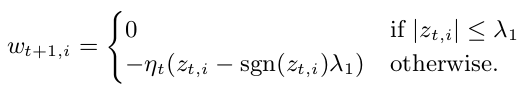
Through a derivation done fairly well in the paper, the weight update step for the proximal algorithm can be done quickly with the intermediate state \(\textbf{z}_t=\textbf{g}_{1:t}-\sum_{s=1}^t\sigma_s\textbf{w}_s\). Updating the intermediate state is constant-time too.
Per-Coordinate Learning Rates
The extreme sparsity of the situation requires adaptive learning rates: by intelligently choosing a per-feature \(\eta_{t, i}\) rate, we can better balance the exploration-exploitation tradeoff in a situation where we see different features activated at different rates.
The paper’s coin example explains this tersely and cogently, so I won’t replicate it here. By tracking the \(\sum_{s=1}^tg_{s, i}^2\), the sum of squares of the \(i\)-th feature of each gradient, we have a measure for each feature’s activity. Scaling the learning rate inversely with this sum lets us trust a very “active” feature’s past more than its immediate changes (and conversely for dormant features). This has asymptotic improvements in the \(\text{regret}\) metric described above.
Saving Memory at Massive Scale
Google makes it clear the bottleneck with this model is RAM: more features included enable higher accuracy.
Probabilistic Feature Inclusion
You can’t perform standard offline feature bagging to exclude features: this requires performing a write to the data to exclude said features, expensive in an online context. Instead, the first several instances of a feature can be ignored, with a feature only starting to be tracked in the coefficient vector if it passes a probabilistic inclusion barrier.
Poisson Inclusion
A simple randomized form of performing online feature inclusion. Upon activation of an unseen feature, with probability \(p\) include the feature: in expectation a feature needs to appear \(1/p\) times to be included.
Bloom Filter Inclusion
Amending bloom filters to store counts (insert increments a count in each slot for each hash function, delete decrements), if a feature has been inserted \(n\) times (with the potential of false positives), it is added to the model.
I still don’t know what rolling set of bloom filters is for sure. In theory, counting bloom filters support deletion (where a recently-added feature would be removed \(n\) times). Perhaps use of one bloom filter is an issue because hitting the counter limit for each slot means deletion would induce false negatives (we lose information about other features with extra counts being stored). So periodically clearing the filter instead of deleting everything is an option; but the details on this are not fleshed out and it’s unclear what approach Google took. The references don’t reveal much, either.
Nonetheless, feature selection in this manner provides exceptional memory savings with low accuracy loss:
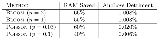
Encoding Values with Fewer Bits
Due to the range of coefficients that were being dealt with, encoding values as fixed-point 16-bit decimals was possible, with no measurable accuracy losses. Over 64-bit floats, huge savings.
Training Many Similar Models
- Using a previous model as the prior saves on training.
- Training multiple models at once coalesces metadata (hash table for weight coefficients only uses one key for many models).
- Count-based learning rates lets Google keep aggregate statistics of number of positives and total examples seen, which can be shared for simultaneously-trained models.
A Single Value Structure
When training multiple models with shared sets of features at the same time, it was efficient to consolidate the weights for the shared variables. Training would work by performing averaged feature updates across models with the same set of coefficients. A bit field keeps track of which coefficient is active where.
This would only seem valid with a Naive-Bayes like assumption for the features.
Computing Learning Rates with Counts
While not quantified, this method makes the assumption that for any event \(\textbf{x}_i\), the activation of feature \(f\) gives a constant probability of click-through: \[ \mathbb{P}(\text{click}(\textbf{x}_i)| x_{i, f}=1)=\frac{P_f}{N_f+P_f} \]
In the above, \(P_f,N_f\) represent the positive and negative examples for events feature \(f\) activated in the past.
Effectively, this makes a Naive-Bayes assumption for adaptive learning, but doesn’t make the harsh non-interaction assumption for actual prediction.
Subsampling Training Data
Click-through happens very infrequently, much less than 50% of the time. For this reason, just training on all the data evenly would lead to a model that is much more educated in the negatives than the positives. By subsampling negatives by some rate \(r\) and magnifying their gradients by \(1/r\) overall validity of the model can be maintained in terms of expected loss, but we also have the nice property that the probability we are correct given we have a true positive is the same as that for a true a true negative.
Evaluating Model Performance
Progressive Validation
Use relative changes (compared to some initial baseline) in all performance metrics to achieve stability.
Deep Understanding Through Visualization
Confidence Estimates
Because of the lack of linear algorithms for confidence estimates, a proxy based on the upper bound of model prediction change is used. \[ \left\vert\textbf{x}\cdot\textbf{w}_{t}-\textbf{x}\cdot\textbf{w}_{t+1}\right\vert \]
This proved “highly correlated” with actual confidence intervals in log-odds space using bootstrap for ground truth.
Calibrating Predictions
As a sort of stop-gap measure, the model’s average prediction rate \(\hat{p}\) over a batch of inputs is compared to the true rate of click-through, \(p\). If there’s systematic bias in the model, it’s corrected by an additional isotonic regression fitting \(\hat{p}\) to \(p\).
Automated Feature Management
Unsuccessful Experiments
Feature Hashing
Using a hash to represent features instead of strings is a memory-saving trick that worked well in other contexts, but required too large of a dimension for the hashtable to be applicable (since collisions hurt accuracy).
Dropout
Dropout is useful for vision but not here because in vision there is a dense amount of redundant information.
Feature Bagging
Feature Vector Normalization
Notes
Observations
- Fundamentally, it looks like RAM is the bottleneck to more AUC improvement: more RAM means more features, more features apparently always helped in the heavily regularized setting.
- You can take a lot of seemingly required assumptions for online algorithm metadata, but still maintain accuracy.
- Amazingly, the single value structure did not worsen performance. I was surprised that two different models, only one of which has a feature with a strong correlation with a shared feature, wouldn’t have antagonistic gradient updates for the shared feature.
Weaknesses
- Certain recommendations seem unapplicable outside of companies with huge amounts of resources:
- New floating point values? That must’ve been a whole re-write.
- Exploring such a large space of approaches takes a lot of people and a lot of machines. There were probably a lot of failed approaches that didn’t make it to the paper: to what extent is the approach presented here “overfit” to CTR prediction? Some of the “failed approaches” even mentioned in the paper don’t have a good explanation behind them, which is indicative of the aforementioned problem.
- It’s unclear what lead to using count-based learning rates or prediction calibration - how much did these methods hurt accuracy.
- How was distributed model training performed? Was parallelism at the per-model level (apparently not completely, with the single value structure)?
Strengths
- Naive Bayes can be safe assumption when learning how adaptive to be for feature rates.
- Insane RAM savings through multiple ingenious, well-engineered solutions.
- Simple methods are made predictive at scale.
Takeaways
- To what degree do our non-Google problems, as readers, have such a large feature space? What can we adopt in systems from here when we have to deal with different tradeoffs?
- Probabilistic feature selection is a novel, online method for both reducing noise and RAM use. It can definitely be used elsewhere.
Open Questions
- Maybe we can’t solve the regret bound for the adversarial case where arbitrary differentiable convex loss functions are presented to us. However, we know \(\ell_i\) take a log-loss shape always. Perhaps there exists an analytic solution to the exact FTRL problem: \[ \textbf{w}_{t+1}=\underset{\textbf{w}}{\mathrm{argmin}}\;\; \eta_t\sum_{i=1}^t\left(\ell_i(\textbf{w})-\ell_i(\textbf{w}_{t}^*)\right) +R(\textbf{w}) \]
- The paper cites AdaGrad and Less Regret via Online Conditioning for a theoretical treatment of adaptive learning. However, these are general FTRL results. Perhaps there is an interaction with the particular FTRL-Proxmal regularization that can yield more specific insights into regret guarantees with an adaptive approach there? To some extent, sparsity and adaptive subgradient approaches seem at odds: the former may make the latter slow to recognize new trends in features.
- What is a rolling set of bloom filters?
- At what point does engineering to be memory efficient become more expensive than just purchasing computers with more RAM?