FAISS, Part 2

I’ve previously motivated why nearest-neighbor search is important. Now we’ll look at how FAISS solves this problem.

Recall that you have a set of database vectors \(\{\textbf{y}_i\}_{i=0}^\ell\), each in \(\mathbb{R}^d\). You can do some prep work to create an index. Then at runtime I ask for the \(k\) closest vectors in \(L^2\) distance.

Formally, we want the set \(L=\text{$k$-argmin}_i\norm{\textbf{x}-\textbf{y}_i}\) given \(\textbf{x}\).

The main paper contributions in this regard were a new algorithm for computing the top-\(k\) scalars of a vector on the GPU and an efficient k-means implementation.

Big Lessons from FAISS

Parsimony is important. Not only does it indicate you’re using the right representation for your problem, but it’s better for bandwidth and better for cache. E.g., see this wiki link, HNSW on 1B vectors at 32 levels results in TB-level index size!

Prioritize parallel-first computing. The underlying algorithmic novelty behind FAISS takes a serially slow algorithm, an \(O(n \log^2 n)\) sort, and parallelizes it to something that takes \(O(\log^2 n)\) serial time. Unlike serial computing, we can take on more work if the span of our computation DAG is wider in parallel settings. Here, speed is proper hardware-efficient vectorization.

The GPU

The paper, refreshingly, reviews the GPU architecture.

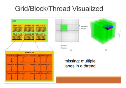
Logical compute hierarchy is grid -> block -> warp -> lane (thread)

Memory hierarchy is main mem (vram) -> global l2 -> stream multiprocessor (SM) l1 + shared mem, going from multi-GB to multi-MB to about 16+48 KB.

There might be one or more blocks scheduled to a single streaming multiprocessor, which is itself a set of cores. Cores have their own floating point processing units and integer units, but other supporting units like the MMU-equivalent are shared.

My takeaways from this section were the usual “maximize the amount of work each core is doing independently, keeping compute density high and memory accesses low, especially shared memory”, but with two important twists:

• GPU warps (gangs of threads) exhibit worse performance when the threads aren’t performing the same instructions on possibly different data (warp divergence).
• Each thread is best kept dealing with the memory in its own lane (which typically is a slice of a 32-strided array that the block is processing with multiple warps in a higher granularity of parallelism), but there can be synchronization points through the register file which exchange memory between the threads.

Note there are 32 threads to a warp, we’ll see that come up.

FAISS = IVF + ADC

FAISS answers the question of “what are the closest database points to the query point” by constructing a 2-level tree. Database vectors are further compressed to make the tree smaller.

Given \(n\) database vectors, we cluster with k-means for the top level, getting about \(\sqrt{n}\) centroids. Then, at search time, we use exact search to find the closest centroids, and then among the closest centroid’s clusters we look for the closest clusters overall.

For a 2-level tree, a constant factor of \(\sqrt{n}\) is the optimal cluster size since then the exact search that we do is as small as possible at both levels of the tree.

Since it’s possible the point might be near multiple centroids, FAISS looks at the \(\tau\) closest centroids in the top level of the tree, and then searches all cluster members among the \(\tau\) clusters.

So the larger search occurs when looking at the second level.

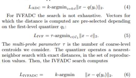
Compression reduces I/O pressure as the second-level’s database vectors are loaded. Furthermore, the specific compression algorithm chosen for FAISS, Product Quantization (PQ) enables distance computation on the codes themselves! The code is computed on the residual of the database vector \(\textbf{y}\) from its centroid \(q_1(\textbf{y})\).

The two-level tree format is the inverted file (IVF), which is essentially a list of records for the database vectors associated with each cluster.

ADC, or asymmetric distance computation, refers to the fact that we’re using the code of the database vector and calculating its distance from the exact query vector. This can be made symmetric by using a code for the query vector as well. We might do this because the coded distance computation can actually be faster than a usual Euclidean distance computation.

FAISS, the easy part

The above overview yields a simple algorithm.

1. Compute exact distances to top-level centroids
2. Compute ADC in inverted list in probed centroids, generating essentially a list of pairs (index of probed database vector, approximate distance to query point)
3. The smallest-\(\ell\) by the second pair item are extracted, for some \(\ell\) not much larger than \(k\). Then the top \(k\) among those is returned.

The meat of the paper is doing these steps quickly.

Fast ADC via PQ

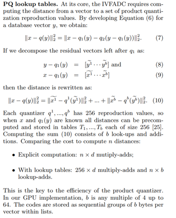
Product Quantization (PQ) boils down to looking compressing subvectors independently. E.g., we might have a four-dimensional vector \(\textbf{y}=[1, 2, 3, 4]\). We quantize it with \(b=2\) factors as \([(1, 2), (3, 4)]\). Doing this for all our vectors yields \(b\) sets of smaller vectors. The FAISS paper denotes these subvectors as \(\textbf{y}^1=(1, 2), \textbf{y}^2=(3, 4)\).

We then cluster the \(b\) sets independently with 256 centroids. The centroids that these subvectors get assigned to might be \(q^1(\textbf{y}^1)=(1, 1), q^2(\textbf{y}^2)=(4, 4.5)\), which is where the lossy part of the compression comes in. On the plus side, we just encoded 4 floats with 2 bytes!

This compression technique is applied to the residual of the database vectors for their centroids, meaning we have PQ dictionaries for each centroid.

The key insight here is that we can also break up our query vector \(\textbf{x}=[\textbf{x}^1, \cdots, \textbf{x}^b]\), and create distance lookup tables on the sub-vectors individually, so the distance to a database vector is just a sum of \(b\) looked-up values!

Top-k

OK, so now comes the hard part, we just did steps 1 and 2 really fast, and it’s clear those are super parallelizable algorithms, but how do we get the top (smallest) \(k\) items from the list?

Well, on a CPU, we’d implement this in a straightforward way. Use a max-heap of size \(k\), scan through our list of size \(n\), and then if the next element is smaller than the max of the heap or the heap has size less than \(k\), pop-and-insert or just insert, respectively, into the heap, yielding an \(O(n\log k)\) algorithm.

We could parallelize this \(p\) ways by chopping into \(n/p\)-sized chunks, getting \(k\)-max-heaps, and merging all the heaps, but the intrinsic algorithm does not parallelize well. This means this approach works well when you have lots of CPUs, but is not nearly compute-dense enough for tightly-packed GPU threads, 32 to a warp, where you need to do a lot more computation per byte (having each of those threads maintain its own heap results in a lot of data-dependent instruction divergence).

The alternative approach proposed by FAISS is:

• Create an extremely parallel mergesort
• “Chunkify” the CPU algorithm, taking a big bite of the array at a given time, keeping a “messy max-heap” of a lot more than \(k\) (namely, \(k+32t\)) that includes everything the \(k\)-max-heap would.
• Every once in a while, do a full sort on the messy max-heap.

Squinting from a distance, this looks similar to the original algorithm, but the magic is in the “chunkification” which enables full use of the GPU.

Highly Parallel Mergesort

As mentioned, this innovation is essentially a serial \(O(n\log^2 n)\) in-place mergesort that has a high computational span.

The money is in the merge operation, which is based on Batcher’s bitonic bit sort. The invariant is that we maintain a list of sorted sequences (lexicographically).

1. First, we have one sequence of length at most \(n\) [trivially holds]
2. Then, we have 2 sequences of length at most \(n/2\)
3. 4 sequences length \(n/4\)
4. Etc.

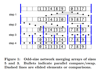
Each merge has \(\log n\) steps, where at each step we might have up to \(n\) swaps, but they are disjoint and can happen in parallel. The key is to see that these \(n\) independent swaps ensure lexicographic ordering among the sequences

This is the odd-merge (Algorithm 1) in the paper. There’s additional logic for irregularly-sized lists to be merged. We’ll come back to this.

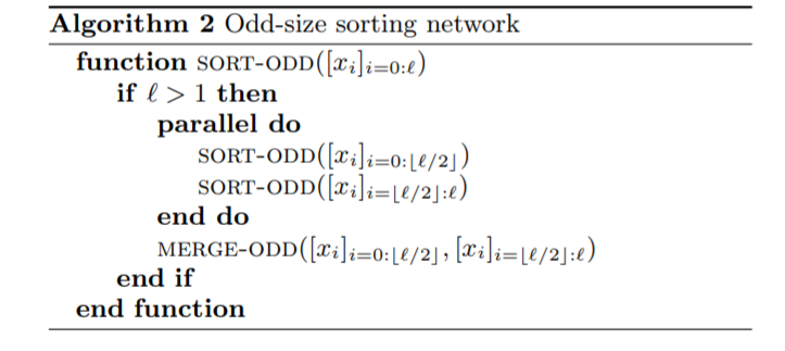
Once we have a parallel merge that requires logarithmic serial time, the usual merge sort (Algorithm 2), which itself has a recursion tree of logarithmic depth, results in a \(O(\log^2 n)\) serial time (or depth) algorithm, assuming infinite processors.

Chunkification

This leads to WarpSelect, which is the chunkification mentioned earlier. In essence, our messy max-heap is a combination (and thus superset) of:

• The strict size \(k\) max-heap with the \(k\) lowest values seen so far. In fact, this is sorted when viewed as a 32-stride array.
• 32 thread queues, each maintained in sorted order.

So \(T_0^j\le T_i^j\) for \(i>0\) and \(T_0^j\ge W_{k-1}\) . So if an input is greater than any thread queue head, it can be safely ignored (weak bound).

On the fast path, the next 32 values are read in, and we do a SIMT (single instruction, multiple-thread) compare on each value assigned to each thread. A primitive instruction checks if any of the warp’s threads had a value below the cutoff of the max heap (if none did, we know for sure none of those 32 values are in the top \(k\) and can move on).

If there was a violation, after the per-lane insertion sort the thread heads might be smaller than they were before. Then we do a full sort of the messy heap, restoring the fact that the strict max-heap has the lowest \(k\) values so far.

• At this point, it’s clear why we needed a merge sort, which is because the strict max-heap (“warp queue” in the image) is already sorted, so we can avoid re-sorting it by using a merge-based sorting algorithm.
  • Finally, it’s worth pointing out that recasting the fully sorted messy heap into the thread queues maintains the sorted order within each lane.
• Further, it’s clear why FAISS authors created a homebrew merge algorithm that’s compatible with irregular merge sizes, as opposed to existing power-of-2 parallel merge algorithms: the thread queues are irregularly sized compared to \(k\) and it’d be a lot of overhead to round the array sizes

This leads to the question: why have thread queues at all? Why not make their size exactly 1?

This points to a convenient piece of slack, the thread queue length \(t\), which lets us trade off the cost of the full merge sort against the per-thread insertion sort done every time the new values are read in. The optimal choice depends on \(k\).

Results

Remember, it’s not apples to apples, because FAISS gets a GPU and modern methods use CPUs, but who cares.

Recall from the previous post the R@1 metric is the average frequency the method actually returns the nearest neighbor (it mayhave the query \(k\) set higher). The different parameters used here don’t matter so much, but I’ll highlight what each row means individually.

SIFT1M

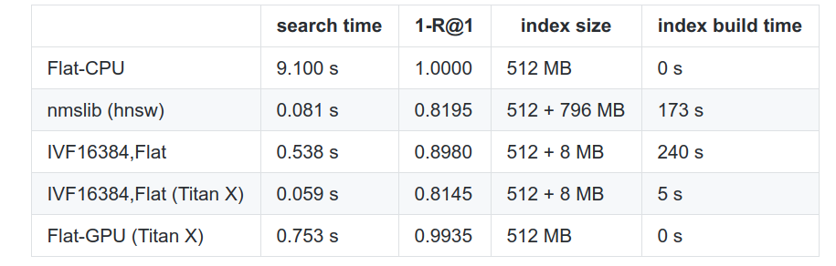
HNSW is a modern competitor based on the CPU using an algorithm written 2 years after the paper. Flat is naive search. In this benchmark, the PQ optimization was not used (database vector distances were computed exactly).

Deep1B

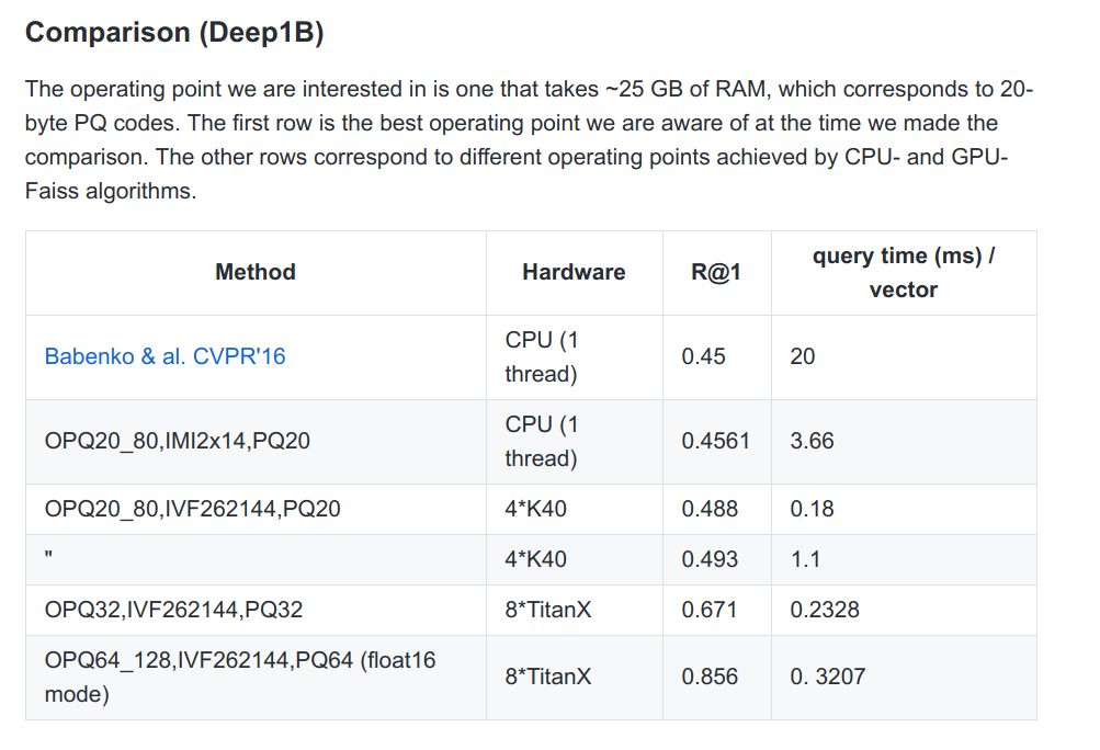
Here, for the very large dataset, the authors do use compression (OPQ indicates a preparatory transformation for the compression).

On the whole, FAISS is still the winner since it can take advantage of hardware. On the CPUs, it’s still a contender when it comes to a memory-speed-accuracy tradeoff.

Extensions and Future Work

The authors of the original FAISS work have themselves looked into extensions that combine the FAISS approach with then newer graph-based neighborhood algorithms (Link and Code).

Other future work that the authors have since performed has been in improving the organization of the two-level tree structure. The centroid based approach of the IVF implicitly partitions the space with a Voronoi diagram. As the Inverted Multi-Index (IMI) paper explores, this results in a lot of unnecessary neighbors being probed that are far away from the query point but happen to belong to the same Vornoi cell. One extension that now exists in the code base is to use IMI instead of IVF.

It’s also fun to consider how these systems will be evolving over time. As memory bandwidth increases, single node approaches (like FAISS) grow increasingly viable since they can keep compute dense. However, as network speeds improve, distributed approaches with many, many CPUs look attractive. The latter types of algorithms rely more on hierarchy and less on vectorization and compute density.